Hello CryoSPARC users! We have just updated the guide with a new case study on EMPIAR 10096. It shows how to recover a high quality 3D map from a dataset that at first glance, appears unusable due to the level of orientation bias present.
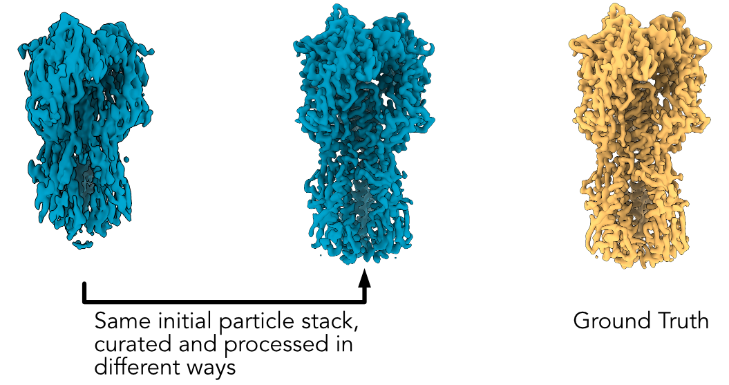
EMPIAR 10096 is a set of movies of purified hemagglutinin (HA) proteins. It is widely considered to suffer from severe orientation bias, producing unusably anisotropic maps. In this case study we detail a processing pipeline that recovers a high-quality, isotropic map of HA from this dataset. Each decision is rooted in an observation of the data and maps themselves, hopefully helping users develop intuition about not only what jobs they may want to run, but why they should run those specific jobs or change those specific parameters.
This case study also provides a theoretical background for understanding why missing views results in anisotropy, which we believe will be useful for all practitioners of single-particle analysis.
I wanted to add that I’ve found it useful to take my latest particle set that has the induced preferred orientation in high-res 3D refinement and rerun ab-initio on that particle set asking for 7-10 classes, with a class similarity factor of 0, and often one of the volumes shows much better orientations. This then works well to go back and do 3D heterogeneous particle filtering with.
Based on the improvement you saw in cFAR using NU-refine, I would guess that optional NU-regularization and adaptive marginalization in heterogeneous refinement would improve the results even further, similar to how BLUSH regularization can help 3D classification in RELION - any chance this could make it onto the roadmap? Would help tremendously for small or elongated particles I think… obviously would be slower but could be very handy for difficult cases
Quick query about this case study @rwaldo - can you get similar results using the 130k particle stack deposited by the authors (Particle-Stack/T00_HA_130K-Equalized-Particle-Stack.mrcs)? Or only when reprocessing starting from repicking the micrographs?
Also, out of interest - if you map the final particle stack back to the 2D classes, where do the particles land? How many of the ultimately useful side views would have been misclassified and lost by 2D classification - or alternatively, how many of the initial “side view” particles selected from 2D actually ended up assigned as side views after rebalancing orientations etc?
I wonder if careful curation either visually using denoised mics or in ice thickness tranches might help draw them out (as an alternative/auxiliary approach to that described in the case study)
I haven’t tried the authors’ deposited particle stack, I’ll give that a whirl later!
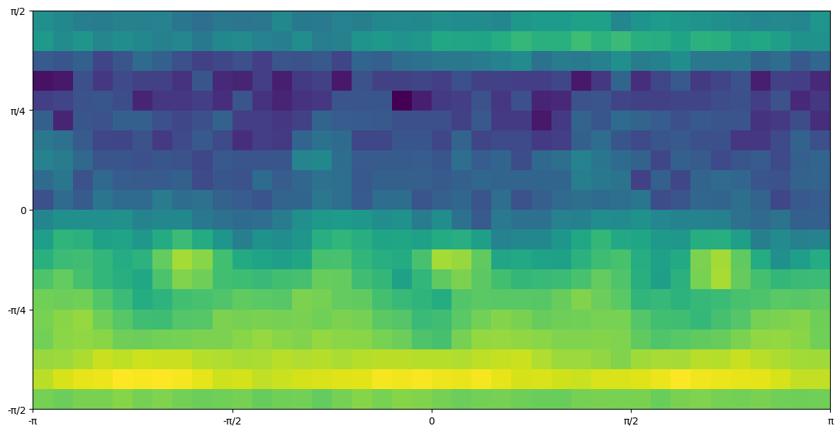
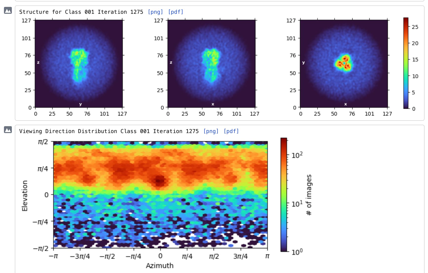
As for your point about individual micrographs, it’s something I hadn’t really considered, but that’s an interesting observation! I looked into this two different ways. For reference, here’s the viewing direction distribution for the particle stack I’m using here.
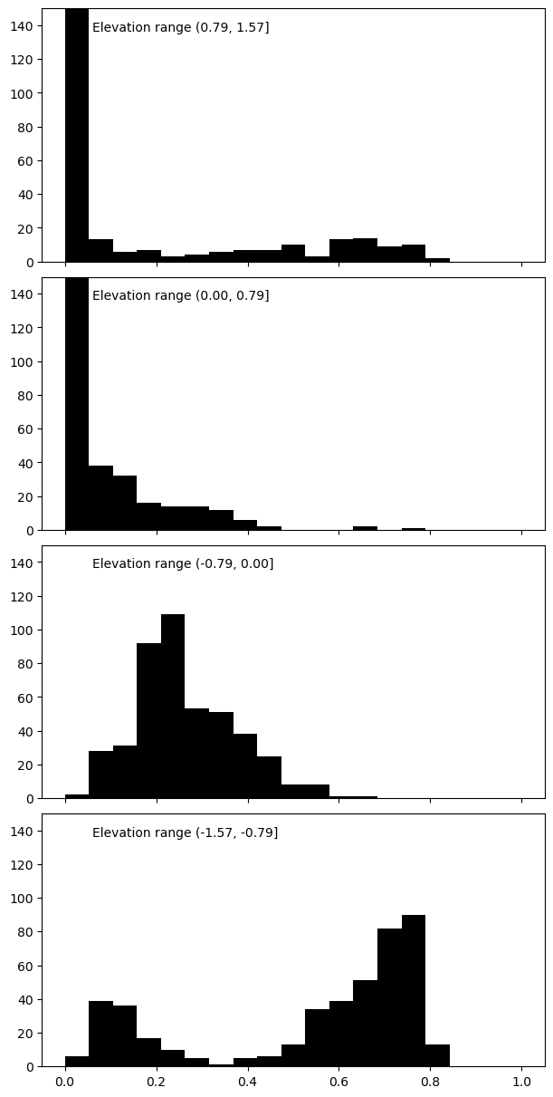
First, I plotted histograms for each quadrant of the elevation viewing direction component (so, near-zero means side view, near π/2 means top view). In each histogram, we are looking at the per-micrograph count of particles which have an elevation in that range:
it seems like (ignoring the strange tendency to see top or top-oblique views as opposed to anything below the equator) side views are fairly evenly distributed, while top views do seem to have a bit of a bimodal shape. Note that I’ve clipped the top two plots’ zero bar, around 300 in each case.
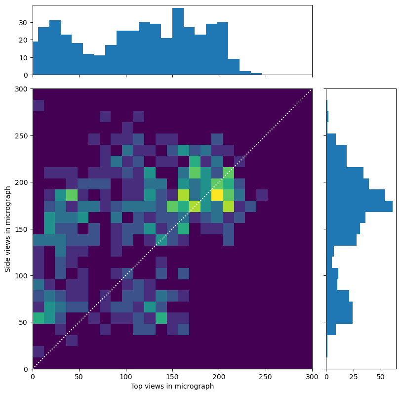
Next, I plotted a histogram where each micrograph has a position defined as:
X: number of particles assigned to a “top” view (elevation > 3π/8)
Y: number of particles assigned to a “side” view (elevation <= 3π/8)
So it does look like there’s a bit of a bimodal distribution of micrographs in terms of how many of each type of view they have, but it doesn’t seem to me that micrographs with more top views have fewer side views or vice-versa. And of course, this all depends on where you draw the top/side cutoff line!
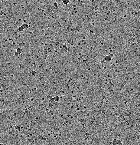
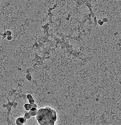
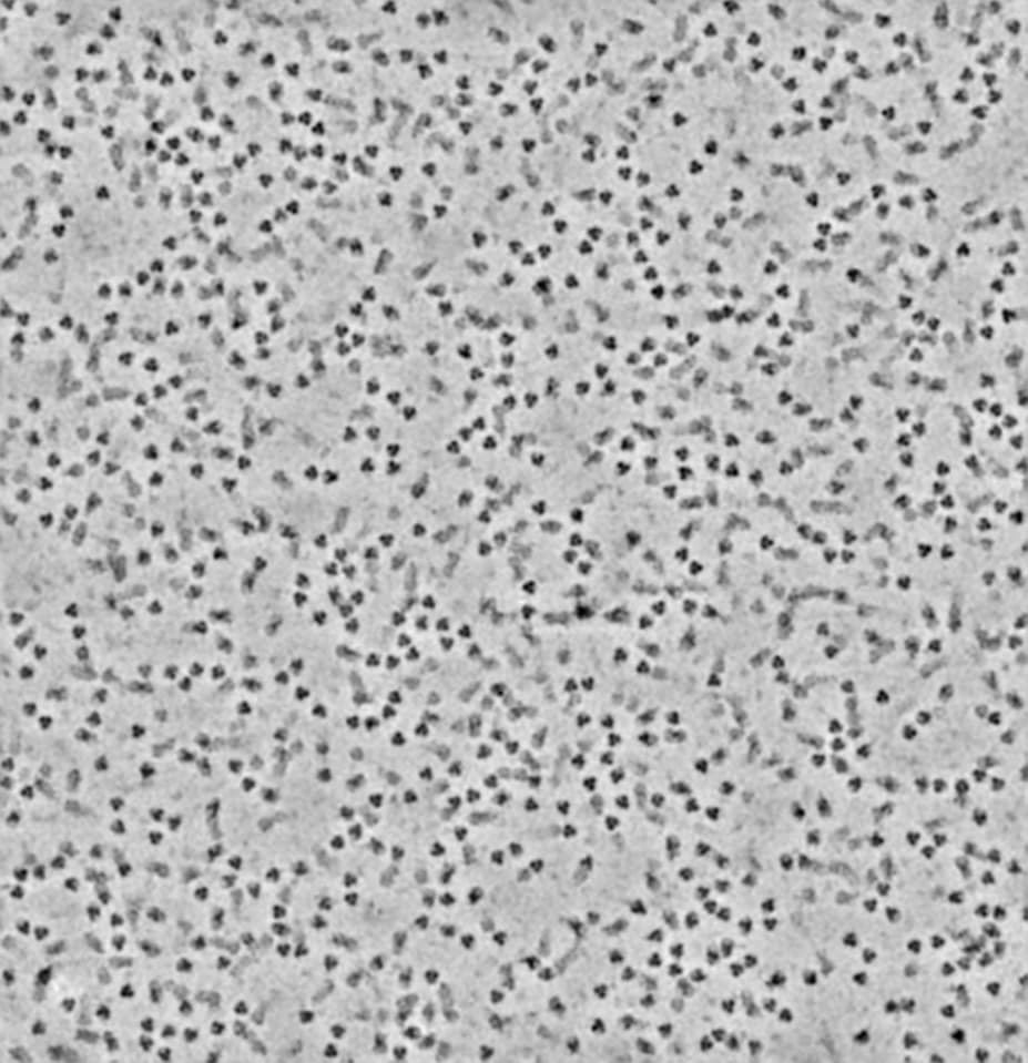
All this is to say I’m not sure I can think of an efficient way to separate micrographs as you suggest, since I personally find side views very hard to tell apart from empty ice, so I’d mostly be relying on how many top views I could clearly identify. I’ll have to keep thinking about it though – this is an interesting idea!
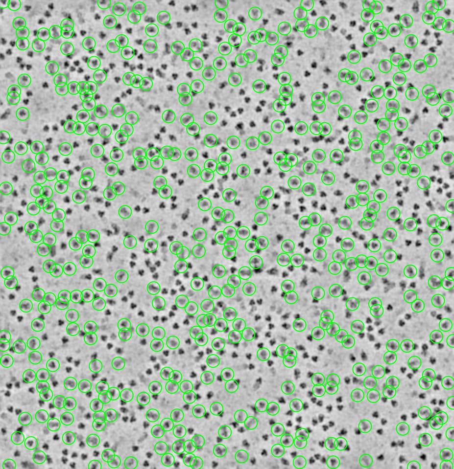
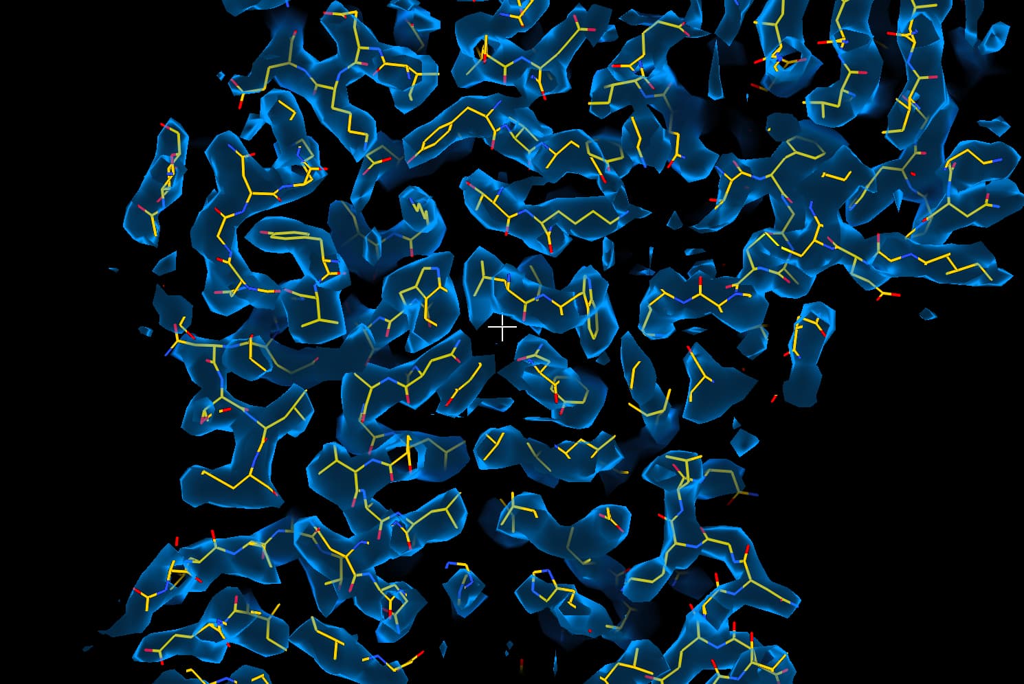
In denoised micrographs you can tell them apart by eye I think - and by then cutting pretty harshly based on local power you can pick them pretty selectively (blob picker ellipitical, min axis 70, max axis 150):
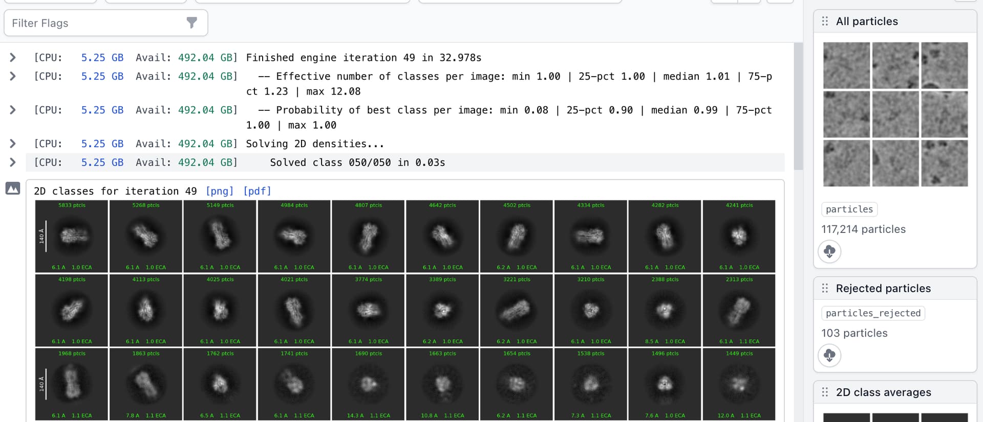
Very much inspired by your case study - I hadn’t expected so much could be squeezed out of this dataset!!
Could probably improve further by tuning the elliptical blob picker or repicking with Topaz…
EDIT:
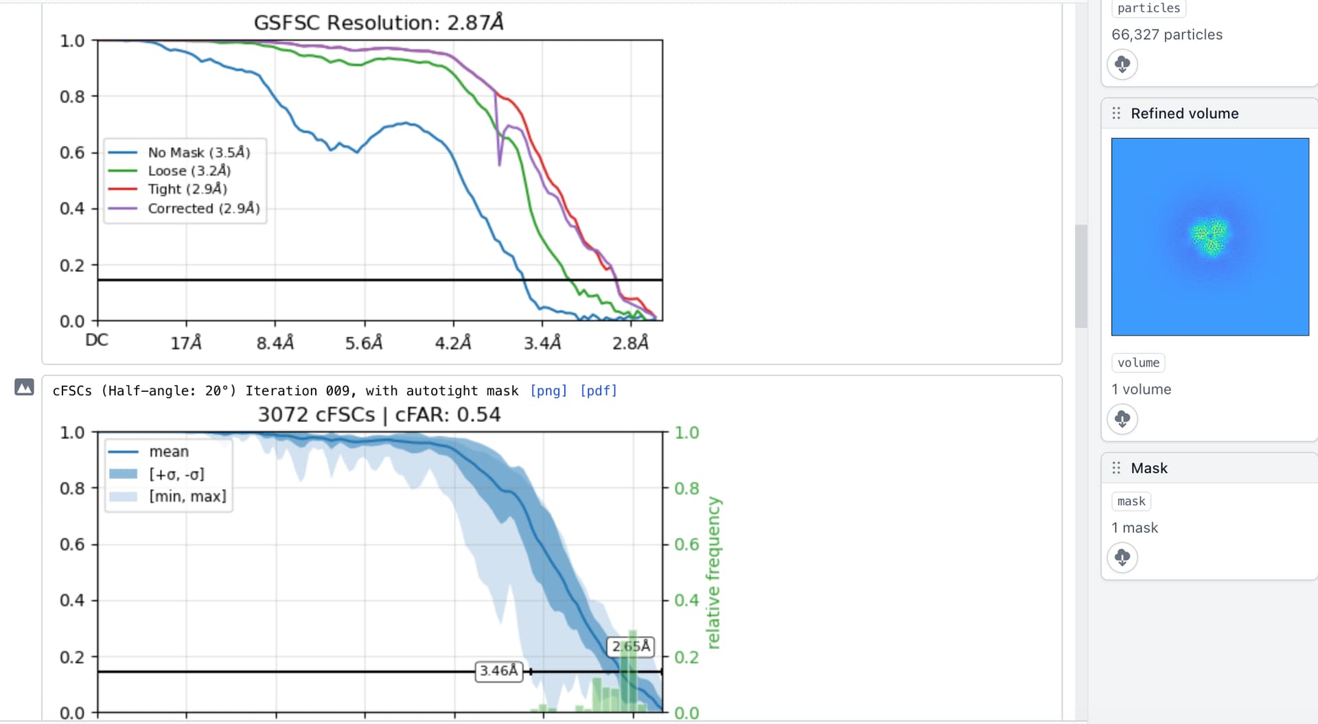
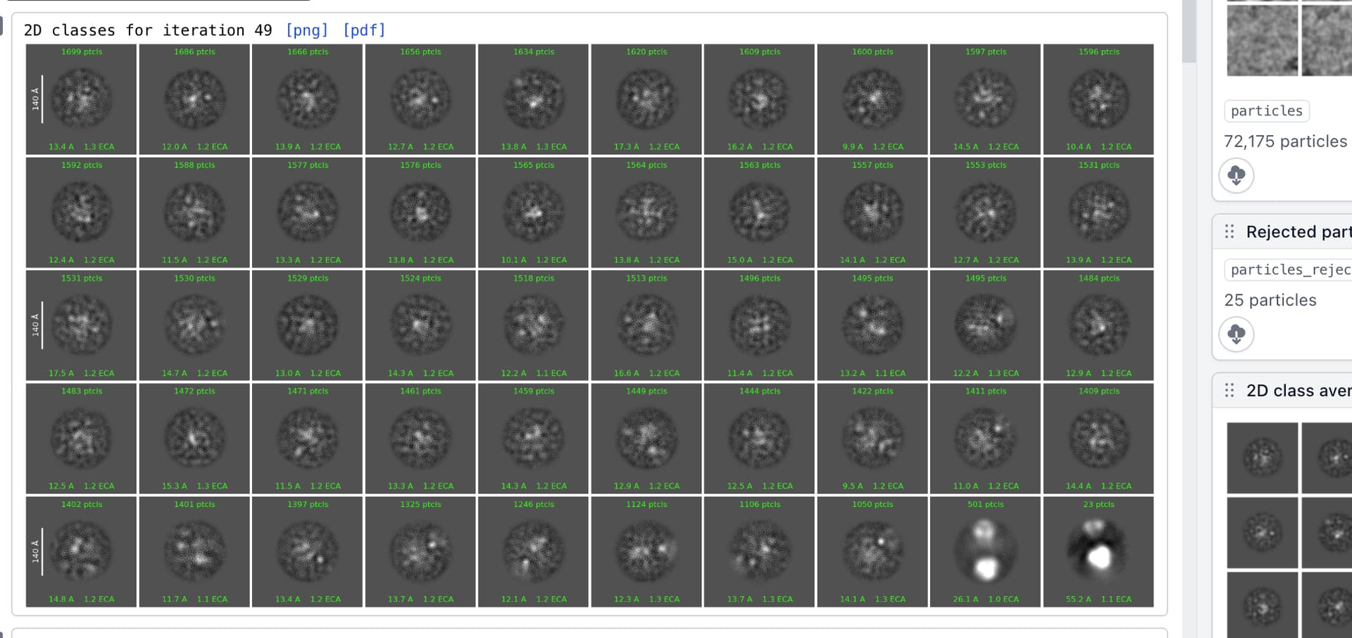
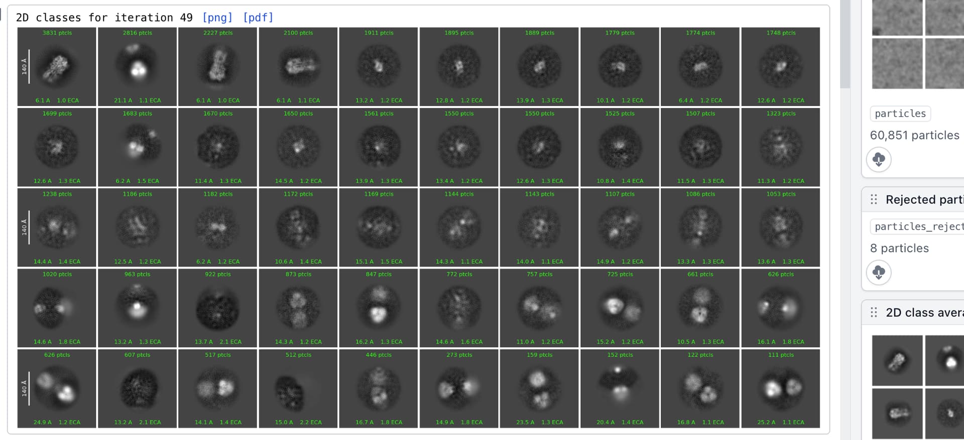
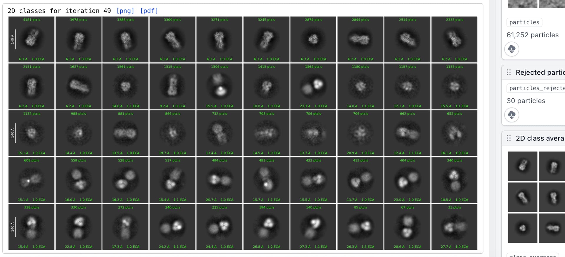
Being slightly more selective with the power thresholds & 2D class selection here gets you to a 62k stack at 3.0 w/ cFAR 0.7; or 42k at 3.1 w/ cFAR 0.8 after orientation rebalancing.
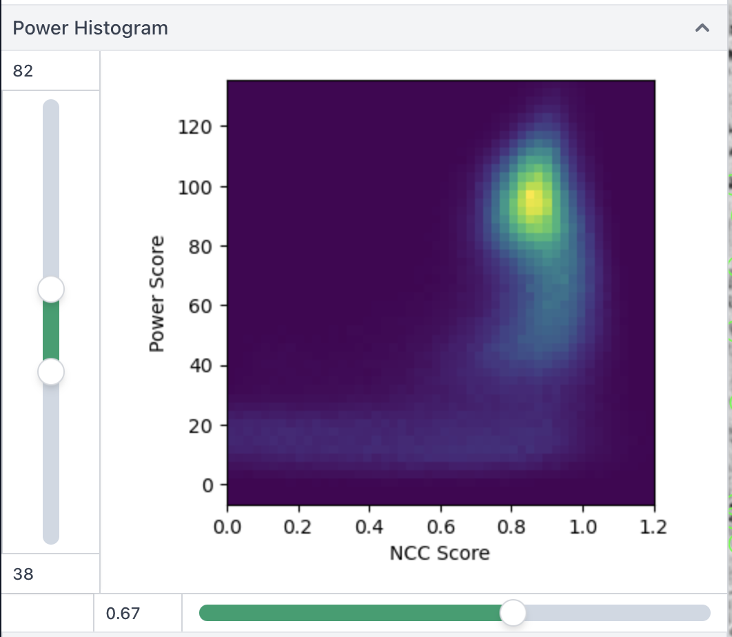
You can actually see it in the inspect picks plot - the side views are the population with lower power (mixed in with empty ice) - the top view occupy the upper “bright blob” at power >80 or so
I didn’t try rebalance orientations on this yet but that would probably improve matters further like you showed
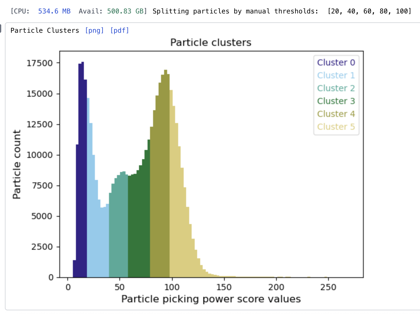
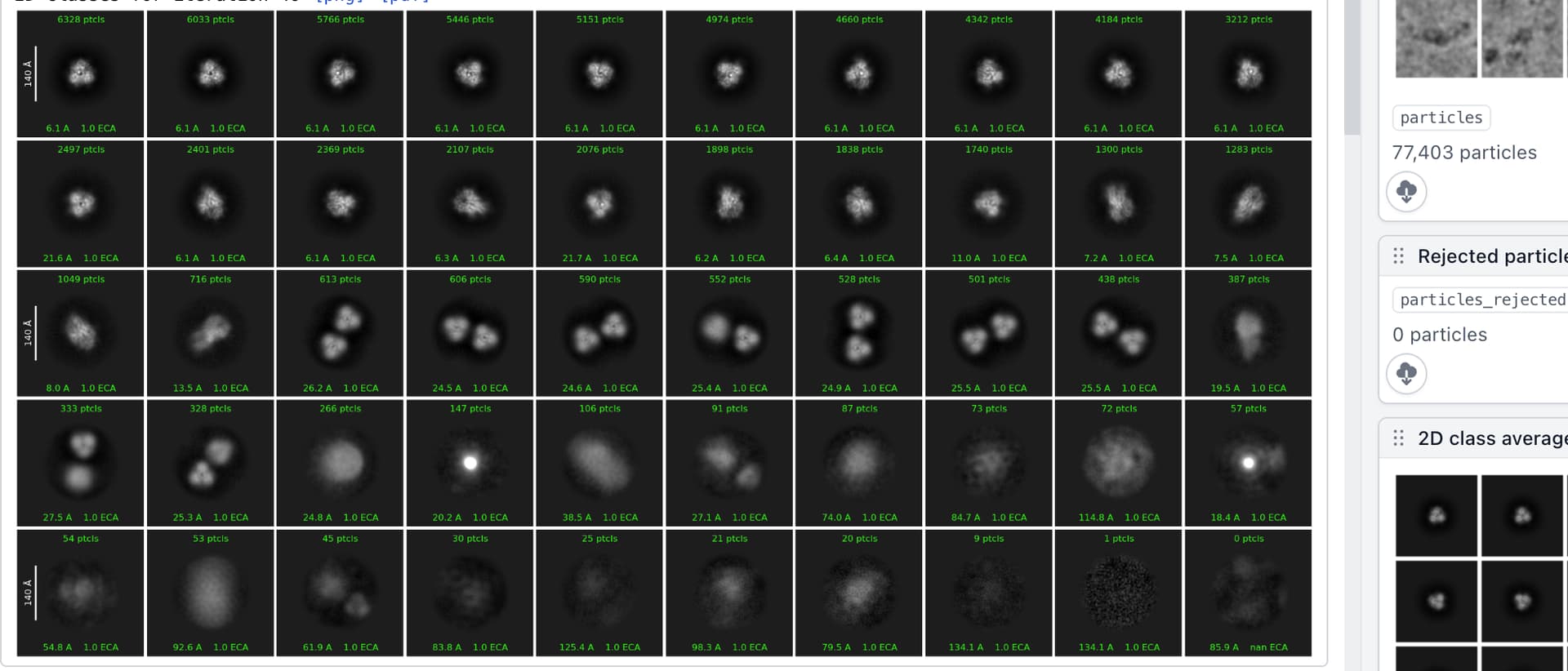
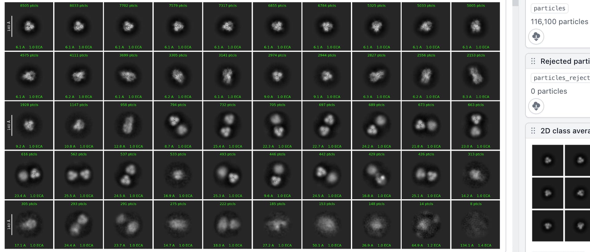
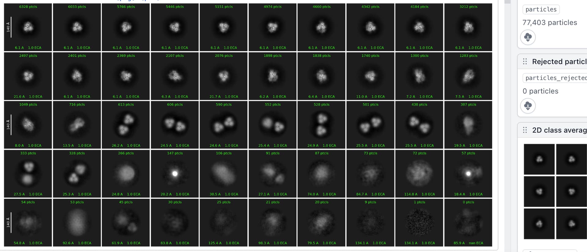
Following up on this a bit, using Subset Particles by Statistic, to split all particles by local power (ignoring NCC), after initial blob picking on denoised micrographs:
You can see there is a very clear trend - the very low power/contrast is junk, a bit higher is side views, and higher again is top & oblique views.
Perhaps this will also be useful as an alternative approach for other samples (obviously will only work if the particle is anisotropic in shape).
Super interesting observation! And indeed this is a potentially useful strategy in cases where different orientations have very different contrasts. When I worked on nucleosomes, I had noticed that what I call the “disc view” is much fainter than the different side views (“gyres view” and “dyad view”, as I ended up calling them).
I have not yet finished reading the case study in details, but wanted to say a big thank you to @rwaldo for taking the time to revisit this dataset and writing this up! This is an excellent example of dealing with a more difficult dataset by using standard tools and careful observations, without tapping into more “black box” tools right off the bat (which is often tempting, but correspondingly often confusing when done with only a vague idea of what the dataset actually contains).