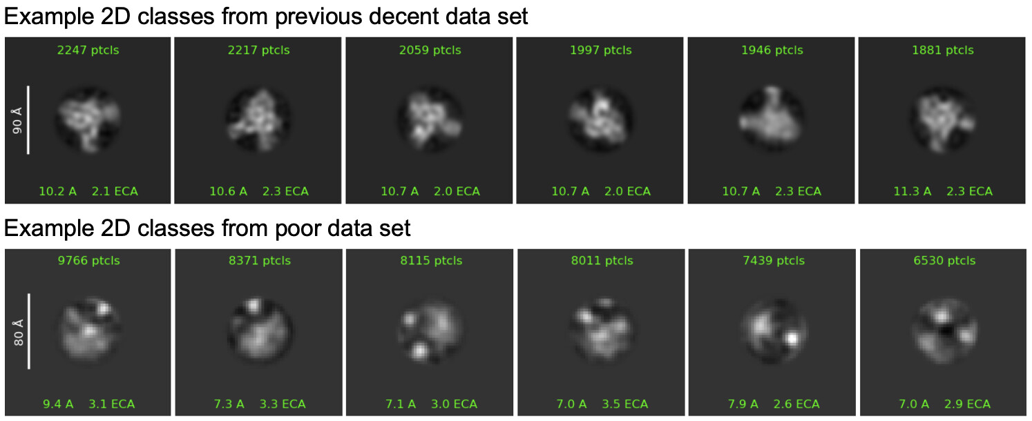
Hello, I am working with a small protein-RNA complex (~65kD total) that we have gotten to 3A resolution in the past, and has been relatively easy to see on denoised micrographs. Several recent Krios collections have, however, been increasingly challenging to get 2D classes from (let alone reasonable ab initio volumes). I am concerned that either motion correction is not working optimally and thus I am losing SNR in my particles, or that denoising micrographs is recognizing my particle as noise. Either way, 2D classes look moderately like my expected complex but are much fuzzier than previous attempts. Could this be due to poor motion correction and what parameters could I consider optimizing for such? Could the denoiser be losing my particles since the contrast is so low? Any and all thoughts are appreciated!
Note: we often see poor contrast in the protein and high contrast from the duplex RNA component of the particles, so it seems plausible that denoising could lead to me not being able to see the particles.
Another possibility is the grid, which you don’t mention. Thicker ice, for example. If re-using a grid from which data has already been collected, you’ll see ice building up, and grids made a different time with a different prep, regardless of whether or not blotting conditions are the same will be different.
The smaller the target, the more critical optimising ice conditions is. Despite the marketing, reproducibility is not easy.
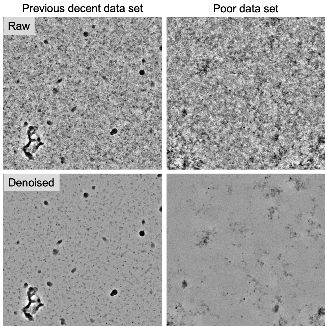
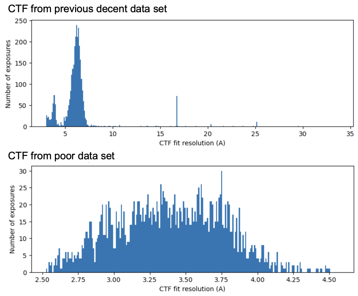
That said, there are various things to check. Look at the global motion for micrographs in the Curate Exposures job. Compare with previous results which were better. If you see a uniform trend toward greater motion, it may contribute. Similarly, check the ice thickness estimate (which are useful but by no means high precision) if estimated ice thickness is elevated, that may contribute. Also check CTF resolution estimates. Compare between datasets. If further support is necessary, a picture says a thousand words - example micrographs from good and bad datasets, denoised examples, 2D classes and the Curate Exposure plots may help further guidance.
Hi @rbs_sci thank you for the response! Excited to be a part of the forum.
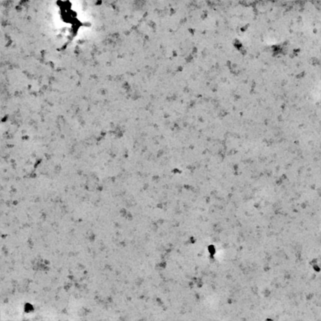
Below is a comparison of a previous data set that gave me a ~4.7Å volume, collected on a Glacios with Gatan K3 detector, and my recent poor data set, collected on a Krios with an Falcon 4i detector.
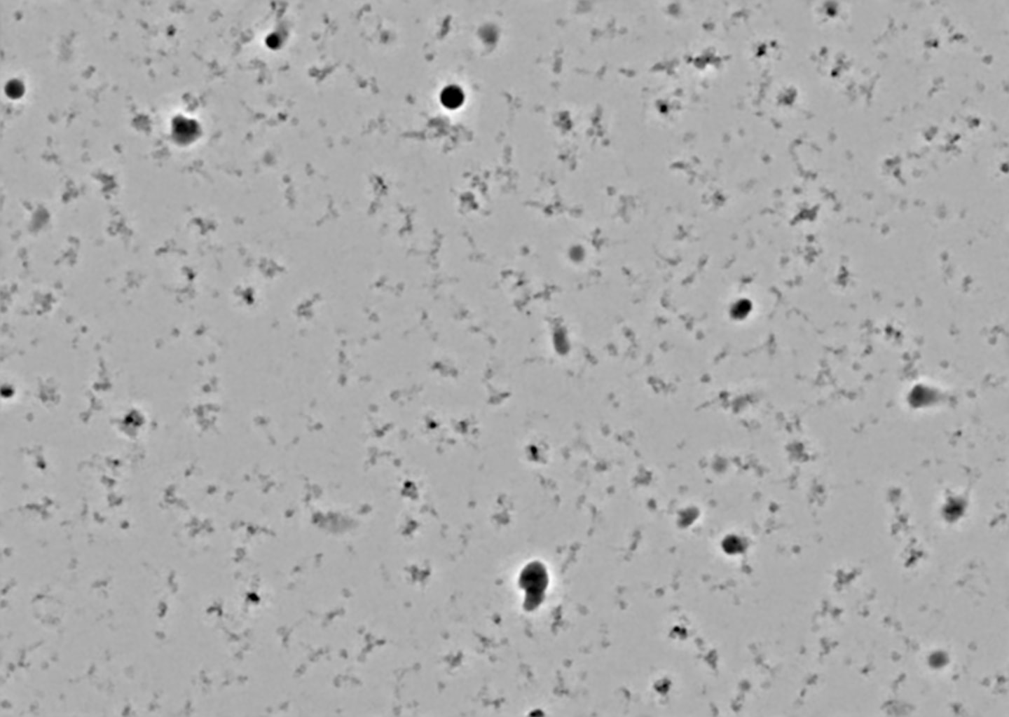
These poor grids are certainly thicker than previous collections. Interestingly, however, my recent collection time was split with collaborators whose grids were thinner (dose on camera of 47e/A^2 to my 44e/A^2, original dose of 50e/A^2) and whose particles are ~300kD, and we are struggling to see their particles too. Below is a comparison of an old data set for their project using the Glacios/K3, which gave us crisp micrographs versus the recent Krios/4i collection, which appears much fuzzier.
This has been a consistent trend over the past several data collections, so perhaps I should also be considering different processing strategies for Glacios vs. Krios collections. This is why I suspect my motion corr or denoising is to blame, I would just be really surprised that the Glacios is truly giving us higher resolution data.
because the Glacios operates at 200 kV and the Krios at 300 kV, a direct comparison of data quality is inherently challenging. Differences seen in downstream processing, including 2D class clarity, reflect not only sample quality but also the underlying imaging physics and optical setup of each instrument.
At 200 kV, electrons interact more strongly with the specimen, leading to increased elastic scattering and stronger phase contrast. For very small particles, this enhanced low-frequency contrast can improve apparent class clarity. This could potentially contribute to the sharper-looking 2D classes from the 200 kV data.
That being said, voltage alone does not explain everything. The ice thickness, objective aperture size, and the use (or absence) of a post-column energy filter can substantially influence contrast, particularly at 300 kV. Other imaging parameters such as defocus range, dose conditions, detector performance, and optical alignment also play important roles in determining final data quality. A meaningful comparison requires careful normalization of imaging conditions. Without controlling these factors, it is difficult to attribute differences data quality solely to ice quality or downstream image processing parameters.
Realistic parameters for data collection of small particles at 300kV: Zero-loss GIF (~20 eV slit), 70 µm objective aperture, defocus range: –1.0 to –2.0 µm, pixel size ~0.9–1.0 Å, ice thickness of 25–40 nm, and strict coma-free alignment. These parameters usually give the best balance between contrast and high-resolution retention.
This looks more like a sample issue. You can see in both the denoised & non-denoised mics that the sample is aggregated and sparse on the right, and well distributed on the left. I don’t think this is a data processing issue.
Harder to say whether this is also the case for your colleague’s example, but unless they are checking the same batch of grids it is not an apples to apples comparison.
Sorry for delay in reply. @olibclarke has you covered I think; saying what I would have done. From mics alone it’s clearly a sample issue. For what reasons, we can only guess. But the poor dataset is clearly aggregated, possibly broken and deeply unhappy.