How to get correct Thon Ring images

Hi!
I’m trying to get Thon Ring images of micrographs using several lines of python code, but the results are not satisfying. As shown in following figures, compared to Thon ring image in published paper (figure 7), my results (figure 1 to 6) are worse and Thon rings are not so obvious. Is there any image processing step missed or wrong? Do you have any suggestion?

Here are details. The data used is from cryosparc tutorial T20S data (EMPIAR 10025 subset).

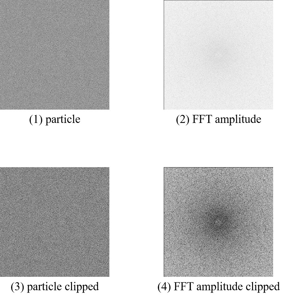
First, I read in the raw movie .tiff file, and sum over frames using numpy.sum(). Then, I read in the gain reference .mrc file, and apply it to summed micrograph by element-wise multiplication. After that, Fourier transformation is perform to the micrograph using numpy.fft.fftshift(numpy.fft.fft2()). Finally, I calculate the amplitude, use Logarithmic function to scale the values with 20*numpy.log(numpy.abs()), and display the result. This results in figure 1.

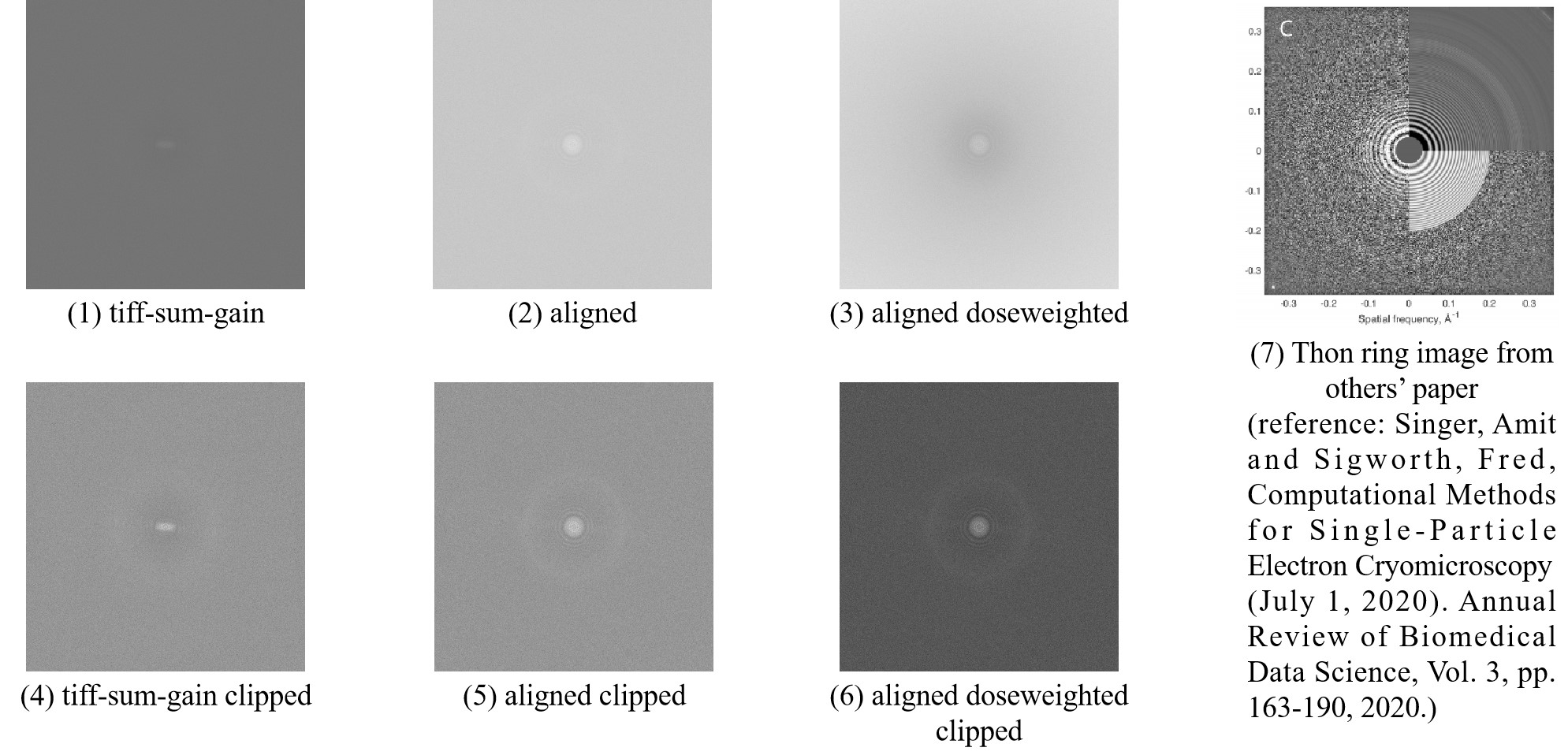
Meanwhile, I try to get Thon Ring images from motion corrected micrographs as well. In the results of cryosparc motion correction job, there are several different files and information for each micrograph (by the way, I’m not so sure what each item means, does any one know?), and I read in both aligned and aligned doseweighted .mrc file. Then, I use numpy.fft.fftshift(numpy.fft.fft2()) to perform Fourier transformation and 20*numpy.log(numpy.abs()) to calculate amplitude. The results are figure 2 and figure 3, respectively.

What’s more, I also notice the contrast_normalization function mentioned in another post (https://discuss.cryosparc.com/t/differences-between-2d-ctf-when-viewed-in-cryosparc-vs-exported-ctf-diag-image-path/10511/6). So I apply this function to figure 1 to 3, and results in figure 4 to 6, respectively. However, all my results have big difference with figure 7, whose Thon ring is more obvious and the entire figure looks more correct.

I don’t know why is the difference. Probably some image processing steps are missed or some steps are wrong? Any one has any advice? Thanks!

Best,
Ciren

1 Like

Oh, I have another question. I start from a picked particle .mrc image, and do the same operation (numpy.fft.fftshift(numpy.fft.fft2()) and 20*numpy.log(numpy.abs())),but I can not see Thon Ring from result images at all, as shown in following figures. Figure 1 is the picked particle (in real space), and figure 2 is the result image of 20*numpy.log(numpy.abs()). I also try the contrast_normalization function for both figure 1 and 2, and result in figure 3 and 4, respectively. As you can see, there is no Thon Ring in figure 2 or 4 at all. Although my Thon Ring images of micrographs above are bad, there are still some ring stuff can be recognized. However, there is almost nothing about Thon Ring in particle FFT amplitude image below. Why is this and what’s wrong? Can any one help me? Thanks!

Hi @CirenSangzhu,

These are great questions! I think your figure 6 is reasonably close to the left half of figure 7 (this is the actual power spectrum, not the fitted CTF). I would try first cropping the power spectrum in figure 6 around just the low frequencies (i.e. +/- 0.35 [1/A], like in figure 7) before passing it to the contrast_normalization function, this might improve the scale a bit more by removing the high freq noise.

To your question, generally particle images don’t show any Thon rings because there is much less signal in a particle image relative to the whole micrograph. I.e. the particle images are swamped with noise, whereas the entire micrograph has enough signal from the diffraction pattern to show Thon rings at the low frequencies.

Best,
Michael

1 Like

Thanks for your response!

Hinted by your advice, I notice that figure 7 only cover the range of +/-0.35 [1/A]. I didn’t notice the axis value before :sweat_smile:. I think your suggestion is reasonable, and I’ll try!

So you mean figure 7 is the result after cropping, only amplitude of low frequencies is shown, while the high frequnecies is absent. Is this a common operation, i.e. most of figure 7-like images appeared in literatures or produced by cryo-EM reconstruction software (some of them may not show the spatial frequency axis value) are actually only the low frequencies part?

Any images like your (7), which is the same as a diagnostic image from CTFFind4, are generated from an entire micrograph. It’s simply not possible to visualize Thon rings in a single particle image, though based on your images perhaps in some cases the first peak could be seen.

PS - I see now in your first post, there is no motion correction. If you sum the frames and then look at the power spectrum, the motion will make the Thon rings weaker. OTOH if you compute power spectra for each frame, and then sum them, the motion effect will be removed due to the shift invariance of the power spectra. Even better would be to combine power spectrum averaging with Welch’s method, where the power spectrum is estimated independently on many smaller windows over the sample and the results are averaged again. Of course, the trade off here is the loss in spectral resolution from using a smaller FT size.

1 Like

Thanks for your advice! I’ll try!

I’m interested in the basic data processing method and computational methods about cryo-EM SPA. However, when I try to write python code to do some simple tasks in cryo-EM data processing, it often fails and can’t get the ideal results. For example, applying CTF to projections, plotting Thon Rings, and other data processing tasks.

Probably I’m not understanding the data of cryo-EM well enough. For example, I don’t know the pixel value range of cryo-EM particle images, how to normalize cryo-EM image data, what difference between cryo-EM images and natural images should be aware of while processing, and what’s the exact meaning of each job parameters in cryosparc, and so on. I believe there must some learning materials about these stuff, but I haven’t find them yet. @DanielAsarnow @mmclean Does anyone have any suggestion? How should I learn these stuff?

Thanks!