Glad my comments were helpful! Continue to call out anything that seems wrong or confusing, as you have been! 
Still, however, I’m not sure why you would want to interpolate to the given box size after reconstruction of each class. Wouldn’t it be both faster and less misleading to simply reconstruct at the particle box size?
Sorry I didn’t say this explicitly before. There is no interpolation after doing a reconstruction. The interpolation takes place during the reconstruction itself. One pixel from a particle image has the coordinates (x, y, 0). This is multiplied by the rotation matrix R for that particle, to find (x’, y’, z’) where to insert into the reconstruction. As x’, y’, z’ are (very likely) noninteger values, we’ll actually look at the rounded down int(x’) and int(x’) + 1, etc. voxels in order to do our interpolations.
If the reconstruction is not the same size as the particle, then we can simply multiply R by the ratio of the sizes (scaling factor) before transforming the coordinates. This same scaling factor also accounts for the change in size due to any zero-padding.
I think we should look more closely and try to figure out whether the inflated FSC really comes from interpolation error or from (Fourier space) smoothness. If it’s the latter, then the FSC isn’t really wrong, but rather the object is just predictable. If it’s the former then the default could perhaps be changed to min(box, 128) instead of 128.
By a non-GS FSC do you mean that the particles are refined together and after refinement simply split into two half-sets, and the half-maps compared?
Correct. I think the original reason not to split half-sets in 3D classification was to keep the effective number of particles larger so as not to miss small classes. FYI Relion doesn’t do this - instead it uses an (also unreliable) SSNR measure to estimate class resolution. You might also be able to turn on half-sets in Relion Class3D using a command line flag (I forget the name, it’s always output by Refine3D).
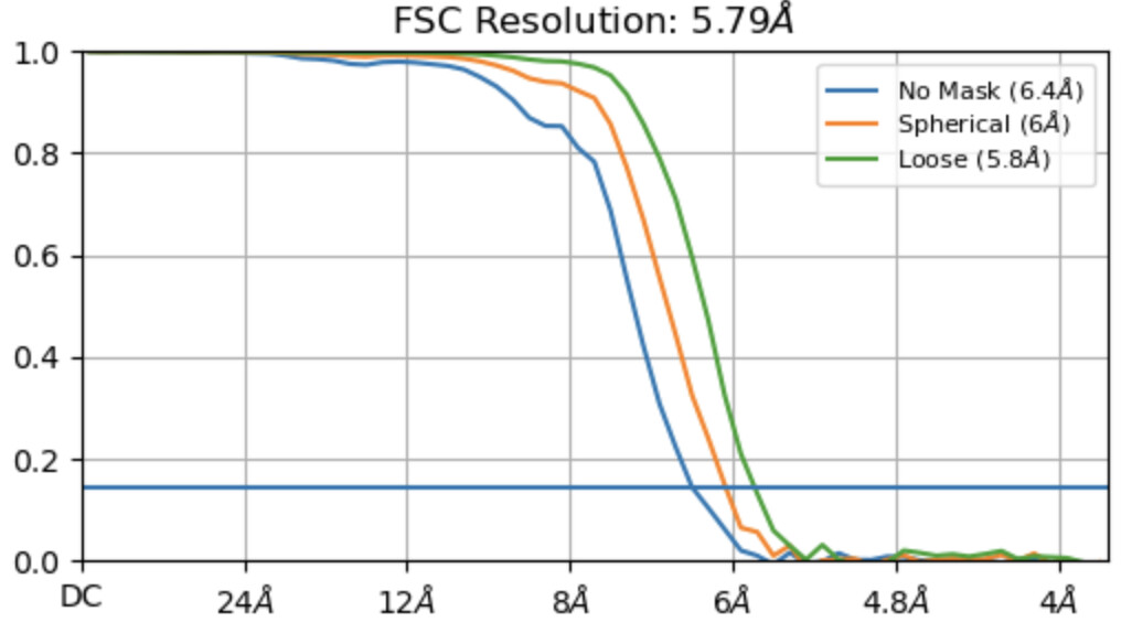
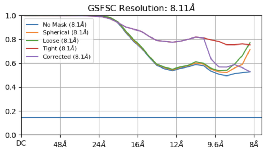
positive asymptotes after the cut-off resolution.
You mean it doesn’t go to zero? Or the curve is step-like? Could you show a picture of what you mean?