I was wondering if anyone knew how the images displayed in jobs like Import Movies and Patch Motion Correction were actually generated by Cryosparc from the raw TIFF images and gain reference. I know how to read the multi-page images themselves into a numpy array in python and how to do the same the with the typical .mrc gain reference files. However, I don’t totally understand what it means to apply that gain reference and what other steps need to be taken to generate images like those in Cryosparc from scratch. If anyone else has done this before, I’d love to hear about how it’s done.
I’m currently working on a project related to beam induced motion of cryo-EM samples, so all my questions are in service of that project. In my initial post I was concerned with how to generate micrograph thumbnails and apply the gain reference, which I’ve since figured out how to do. However, as I’ve been using Cryosparc more, I still have some other questions that someone on the Cryosparc team might be equipped to answer, since I can’t find satisfactory answers online. I would be thrilled if you could answer some of these, even if some of them are unconventional.
To generate thumbnails for the micrographs, I had to sum over the frames of the raw TIFF files and split the image into squares and sum over those before it was remotely human readable. given that any individual frame is so sparse in information (at least to the eye), what does this mean for the accuracy of motion correction, including full frame motion correction? Do we have any idea if this accurately describes stage drift? Also, my understanding is that full frame motion correction essentially does translational cross correlation between frames to determine the likely stage drift. Is this the case?
Similarly, do patch motion correction and local correction simply apply a similar process of translational cross correlation to smaller patches or boxes around picked particles to predict trajectories? I also noticed that the plots produced by local motion correction contain grey lines that are separate from the trajectories plotted in red, and I have yet to find an explanation for what they represent. I was also wandering what biases are involved in predicting the trajectory (for example, biases for smoothness).
The exported exposure.cs file from local motion correction contain a field, ‘background_blob/path’ that points to a set of .mrc files. When I view one of these files, it looks like it’s meant to represent the average shade of the background in any given part of the micrograph. However, the dimensions of the micrograph are not multiples of the dimensions of these files (I’m not sure why this is). I was wondering what these files are and how they’re used by Cryosparc.
I’d appreciate whatever information you could provide related to my questions.
To generate thumbnails for the micrographs, I had to sum over the frames of the raw TIFF files and split the image into squares and sum over those before it was remotely human readable. given that any individual frame is so sparse in information (at least to the eye), what does this mean for the accuracy of motion correction, including full frame motion correction? Do we have any idea if this accurately describes stage drift? Also, my understanding is that full frame motion correction essentially does translational cross correlation between frames to determine the likely stage drift. Is this the case?
Similarly, do patch motion correction and local correction simply apply a similar process of translational cross correlation to smaller patches or boxes around picked particles to predict trajectories? I also noticed that the plots produced by local motion correction contain grey lines that are separate from the trajectories plotted in red, and I have yet to find an explanation for what they represent. I was also wandering what biases are involved in predicting the trajectory (for example, biases for smoothness).
It’s definitely expected that you would have to sum over frames in order to get human-readable thumbnails. Low-pass filtering will also help particles stand out. You’re correct that there’s relatively little information in each movie frame. Cryosparc’s motion correction jobs all estimate a motion trajectory based on optimizing a function that combines trajectory-shifted correlation with some sort of regularization. Because the raw frames are so noisy, it’s likely that correlation alone would just fit to the noise. Local motion, for example, requires that the motion of nearby particles be correlated, and requires that the trajectories meet a certain criterion of smoothness. In the local motion plots you are referring to, the grey lines are what the trajectories would be based on optimizing the correlation alone, without enforcing any correlation or smoothness.
what does this mean for the accuracy of motion correction, including full frame motion correction? Do we have any idea if this accurately describes stage drift?
I suppose I would summarize it as follows: good motion correction of single particle cryo-em data requires striking the right balance between finding the correlations in the data and enforcing certain sanity checks (regularization). Too little regularization and you’ll just fit to the noise. Too much regularization and you’re inventing trajectories based on your preconceived notions of what they should look like (or in extreme cases, getting no motion at all). Fortunately, we can get some sense of whether motion correction is doing the right thing or not by comparing the final reconstruction resolution with different motion correction approaches. You’ll find that in practice it works well, though there are still of course frontiers to explore.
You might also find the following papers interesting:
I’m also interested your question: how to generate micrograph images similar to CryoSPARC Import Movies job, which is human-readable.
I try T20S subset used in CryoSPARC tutorial, but fail to get ideal results. Here is how I deal with the .tiff raw movies.
I use skimage.io.imread to read a .tiff raw movie file in python, and get a numpy array with shape of (38, 7676, 7420). Then, I sum the 38 frames using numpy in python by np.sum(tiffdata, axis=0), and get a numpy array with shape of (7676, 7420). In my understanding, this summed .tiff data should be human readable, at least some particles or other information should be visualable. I convert the data type of the summed tiff data to uint8 (because I find some value exceed 255) by sumdata.astype(np.uint8) and display the result by skimage.io.imshow(sumdata, cmap='gray'). However, the displayed image is just a dark image like this.
I’m wondering what’s wrong and what is the correct way. In the following reply under this post, it seems that you have figured out how to do it in the right way, but I still don’t get it. Could you please give me some advice?
This sounds like a problem related to the color scaling. I suspect that whatever way you’re using to normalize the pixel values is causing them to get displayed as black. I can describe the process I use currently.
Open the raw tiff file as a numpy array.
Sum over frames and bin the images by some factor. (By binning, I mean that you essentially sum over tiny boxes of some pre-determined size across the entire image). Both of these can be done efficiently using numpy methods by reshaping the array and summing over the right axes.
However, during trying to solve this problem, I have some further questions about cyroEM data.
In my understanding, binning can make the result more human readable, but not a step must be done. Am I right? In my .ipynb file, I didn’t bin the image, and particles are visiable, though not so obvious. I haven’t try binning, but according to your description, if I do 2x2 binning in a 1024x1024 image, it will become a 512x512 image. It’s like downsampling the image, probably will make the particles more obvious? And also, @hsnyder@wtempel does cryosparc bin the image to get the thumbnails or images displayed in job UI?
I have also seen “bin” operation somewhere else, but never be really clear about this. What is “bin” operation for? For making the image more human readable, reducing computation cost, or some other reasons? What images should we use to do the following 3D reconstruction, images before or after binning? And how do we perform binning? Besides your description, I have also seen “Fourier crop” somewhere. In my opinion, “Fourier crop” operation transforms an image to Fourier space, crop from center (drop some high frequence information), and then transform back to real space. I’m confused, which way is “bin”, or are both of them ok?
About the contrast normalization, it’s amazing. @hsnyder@wtempel Is it only for visualization, or really operate on the cryoEM data, and the following reconstruction use normalized data? Also, is this operation widely used in cryoEM community, or even something like a standard processing step? In the contrast_normalization function code, there are some parameter like "2nd" percentile, "98th" percentile, extend = 1.5. Are this parameters set according to some common standard in cryoEM?
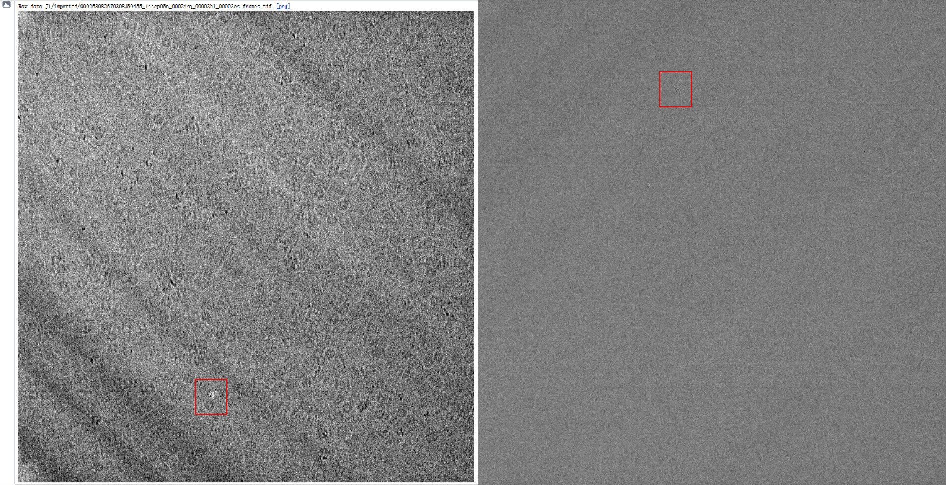
I run my code and get the summed tiff data visualization result. I find that the result I get seems to be the bottom-up flipped (in Y axis) version of the one displayed in cryosparc job UI, as shown in the following figure.
Left one is from cryosparc job UI, and right one is the result of my code. There is a obvious mark in this raw movie (in red rectangle). Obviously, they are bottom-up flipped. Do you also have this problem? Or @hsnyder@wtempel does cryosparc flip the image for visualization inside the import movies job code?
As shown in the figure above, there is still big difference between two results. Cryosparc one is more clear. Do you have this problem? Do you know is it because I didn’t bin the image, or cryosparc applies extra image filtering, or some other reasons?
I am new to cryoEM and there are lots of things about cryoEM data I don’t understand. What’s worse, I find it difficult for me to search information and learn about something really basic about cryoEM data. For example, why are there both positive and negative value in .mrc file of particles or final 3D map, what is the range of cryoEM data in .mrc file (for natural image it’s [0, 255]) and so on. I think I don’t find the right way and right resource to learn these stuff and am confused. So I would really appreciate it if someone can give me some tips on how to learn this stuff.
I mention binning because it tends to make it easier to spot particles and other features, but it’s not fundamentally necessary. As I understand it, both that and the contrast normalization don’t play a role in data processing (The contrast normalization function doesn’t actually alter the arrays or anything; it just gives you parameters for plotting to make the image easier to look at). You’ll probably get a similar result by cutting out the high frequency contributions of the Fourier transform and transforming back, but seeing as the goal is just to make a human-readable image I usually just opt for binning.
Your observation about the image being flipped has to do with how you’re displaying the array. The row of the array corresponds to some y location, but the array is being displayed so that row 0 appears at the top, which means the image appears flipped. If you want to make the two look the same you can either use the numpy.flip function or flip the axis in pyplot (I think there’s a command for that, but I don’t remember how it works).
Thanks for your patient explaination!
I think I get it. All operations like binning, contrast normalization and so on are just for making visualization result more human readable. Just for plotting, not really processing the data. Since it is so, parameters in contrast normalization code and some other questions are not so important.
Your explaination really helps! Thanks a lot!
Binning won’t make particles easier to see. Applying a lowpass filter at [user preferred cutoff] will make particles easier to see as the low frequencies are the larger objects and the high frequencies of the particle are hidden in the noise as well as being delocalised by the effects of the CTF (while modern detectors are better, cryo-EM data still has poor signal-to-noise…)
“Binning”, “downsampling” and “Fourier cropping” are effectively the same thing. Downsampling and Fourier cropping are two different terms for the same thing, but “binning” is slightly more complicated as different fields use the same word and can have subtly different implications (e.g. real space cropping rather than Fourier space cropping). However, in modern cryo-EM image processing, the three are basically interchangeable. At the camera level during acquisition, “binning” is just grouping pixels together, e.g. a 4,096x4,096 pixel sensor would have pixels grouped “2x2” to achieve 2,048x2,048 readout, but that’s another discussion.
Normalisation of the data is required for some cryo-EM processing algorithms (or you get errors) while others do not require it. It’s pretty standard, though, although different processing suites may have subtly different requirements regarding normalisation. A reason for normalisation is to compensate for variations in ice thickness between and across micrographs; if everything is normalised the same (e.g., as RELION wishes with a mean of zero and standard deviation of one) then particles can be treated the same. If I remember correctly, the way CryoSPARC calculates its noise model means that it isn’t quite so bothered about the precise normalisation, but it’s best to try to get everything uniform (one of the CryoSPARC team will correct me if I’m wrong here).
C++ and Python handle arrays differently. It can also depend on the library used. Also, different formats can base their zero point in different places (bottom left, top left, etc…)
The CryoSPARC image looks like the contrast has been boosted and a filter of some sort applied. Perhaps just the latter though.
The MRC format has various different types, which can vary a lot; signed/unsigned, integer/float, real/complex… in cryo-EM right now the most common are float32 and float16. See the CCPEM page about the MRC standard for more information about the MRC format.
Binning is usually done for processing speed early on in the processing pipeline. 2D classification and particle picking do not require extremely high resolution and in fact permitting extremely high resolution can be potentially dangerous due to “fitting to noise”. But ultimately early stage binning is done to speed things up - for example, dropping the sampling frequency from 1 Å to 2 or 3 Å (or lower) won’t negatively impact picking and 2D classification (or early 3D classification) but allows the box size to drop by a factor of four (2x bin) or nine (3x bin) which can significantly reduce storage and memory requirements, along with being much faster to process.