I am expecting preferential orientation for the top and bottom views (based on particle distribution in 2D classes), but the results seem to suggest that the side views are preferred. How are the spherical plots presented, relative to the 3D volume?
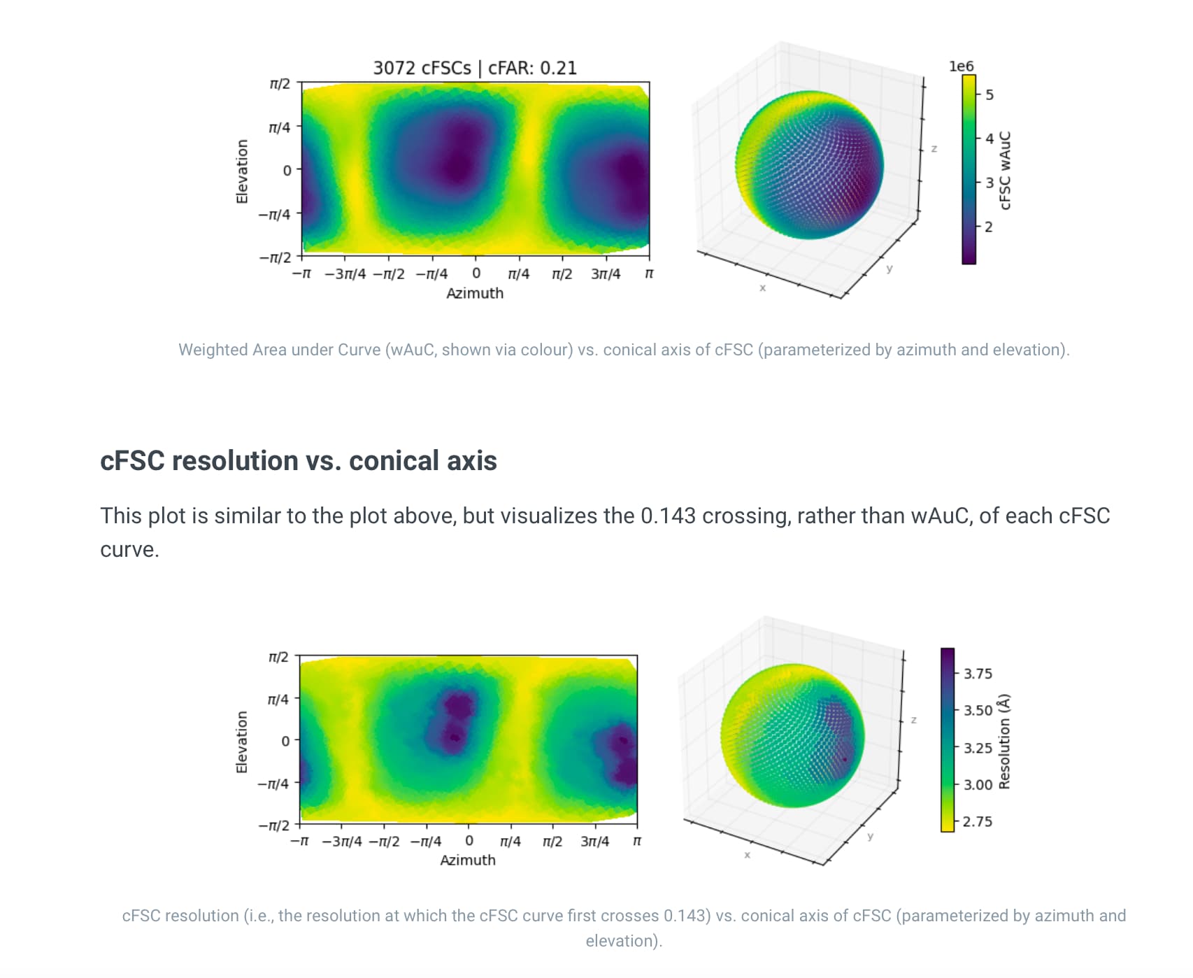
Basically, higher conical FSC resolution correlates with the cFSC wAuC in your figure - so the higher (more yellow) regions of your plot have better directional resolution.
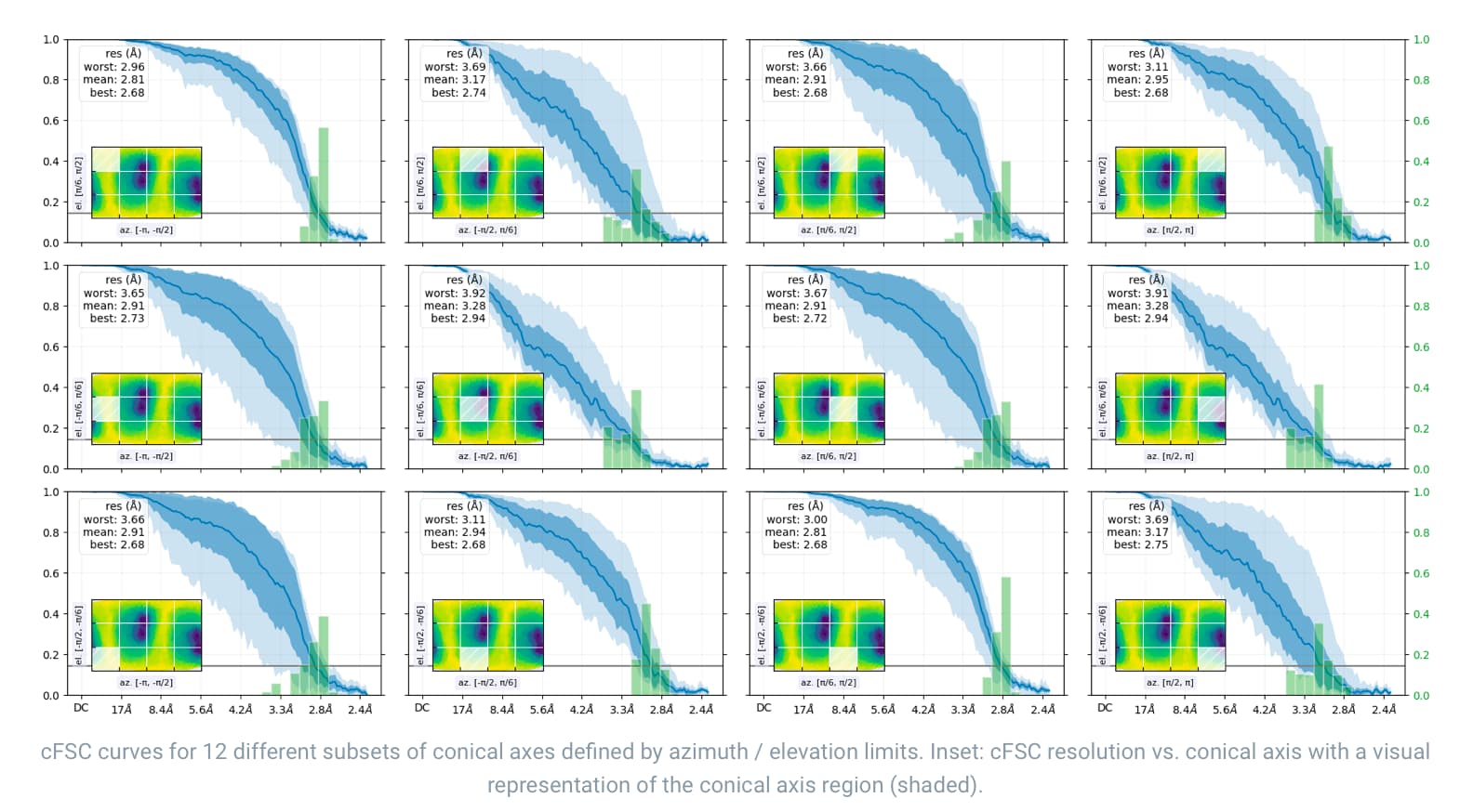
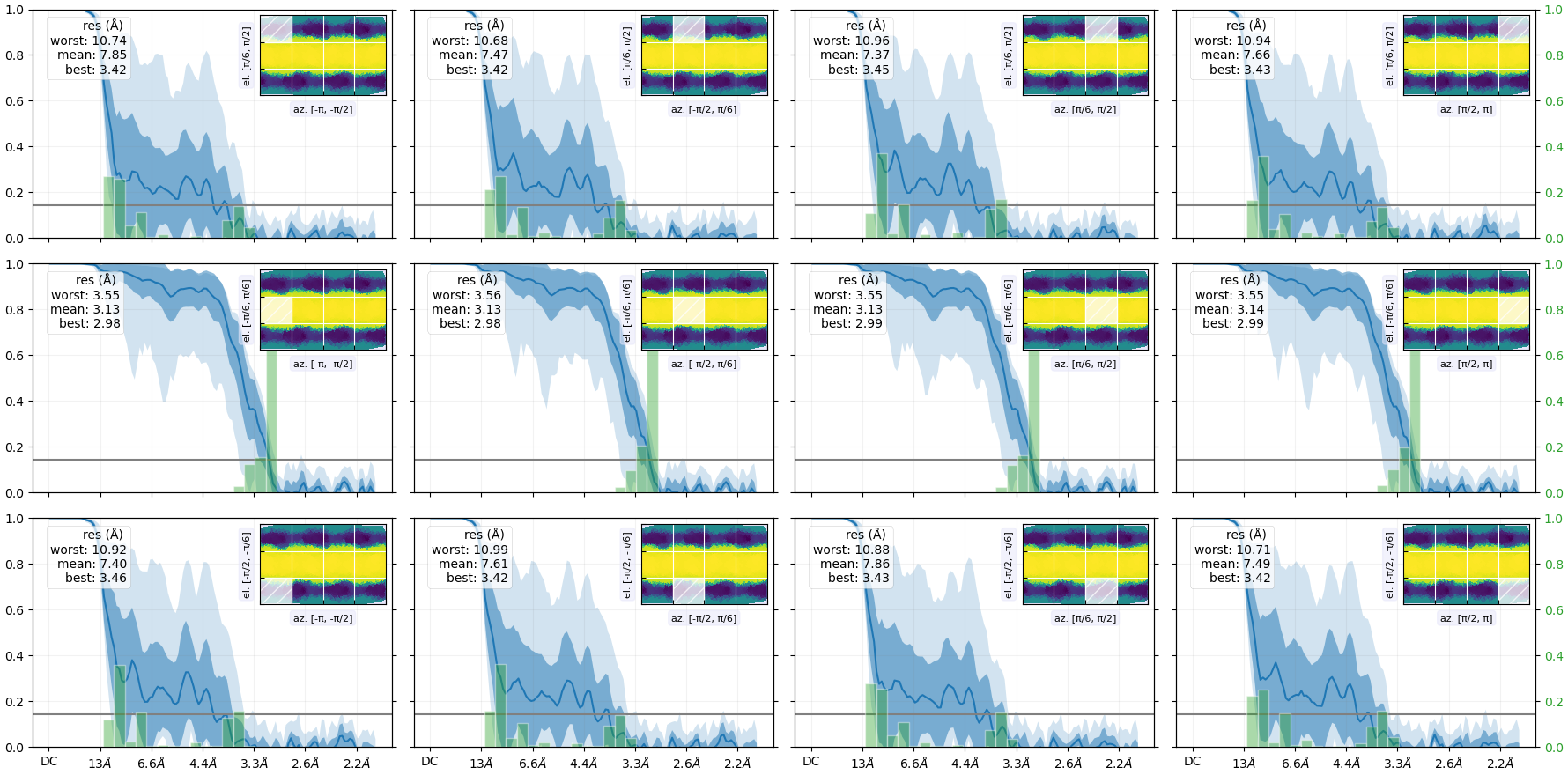
Or in other words, assuming your side views are along the equator (Elevation=0), the side views have better directional resolution than the top views. There should be another plot somewhere in your log with per-region conical FSCs, which may be helpful in interpreting this plot:
I believe the orientation of the elevation/azimuth figure should be the same as what you have for the orientation distribution from the preceding refinement, if that helps?
EDIT:
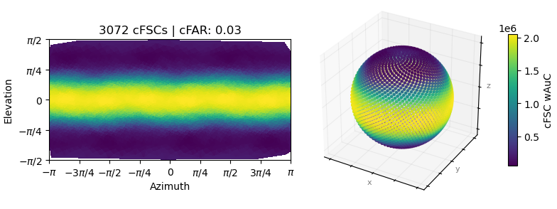
Now I am confused too - this is the example plot for the HA trimer from the guide, which predominantly has top views, and the side views are definitely along the equator:
Thanks for your reply. I understand the directional resolution part, but the results don’t correlate well with my last refinement.
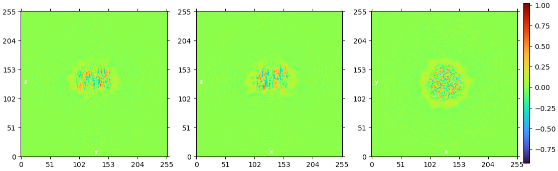
The map from the Non-uniform refinement job I used as the input had some “stretching” of the density when looking at the side views. The top views have noticeably better resolution compared to the side, which is the opposite of what the orientation diagnostics suggest.
Yes I see what you mean - what does the “grid” of example directional FSCs in the Orientation Diagnostics log look like? Does it match what you expect from the plot?
I am expecting preferential orientation for the top and bottom views (based on particle distribution in 2D classes), but the results seem to suggest that the side views are preferred. How are the spherical plots presented, relative to the 3D volume?
These wAuC / 0.143 threshold plots are spherical plots with respect to the ‘conical axis’ of the cFSC, which is distinct from the viewing direction. We have a note about this in the tutorial, which I’ll quote here:
Although they can both be represented via azimuth and elevation angles, the conical axis of a cFSC should be carefully distinguished from viewing direction. Concretely, low cFSC values along a particular conical axis do not imply that more views are necessary from that direction. This is due to the fact that a particle contributes Fourier information to a Fourier slice whose components are orthogonal to the viewing direction…
In this case, the wAuC plot shows poor cFSC values for conical axes at the poles – this does indeed correspond to the case where there are very few side views, and many top/bottom views, as expected from your particles. This is also the case for the untilted HA Trimer, which has a very similar cFSC distribution in axis-space, as Oli noted.
In Fourier space, the dominant top views contribute to a ‘slab’ with a roughly vertical normal. This slab will fill in cones that are ‘horizontal’, and hence result in higher FSCs along the equator in axis space. The same slab will also result in ‘vertical’ cones being largely empty, and lead to the poor resolutions at the poles (again, in axis space). This is definitely confusing at first, since this is ‘orthogonal’ to the quality of 2D classes. Perhaps one way to build intuition here is to identify axes with poor cFSC values with the direction of ‘stretching’ / smearing in the map.
Hopefully that makes sense. Appreciate any suggestions for ways we can make this clearer in the plots.
Thank you for the explanation, that makes sense now!
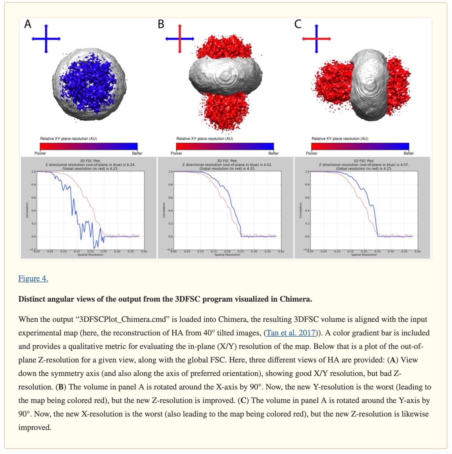
In the 3D-FSC plotting tool for Chimera, the authors address this by plotting the resolution in the plane orthogonal to the direction of the cone, e.g. see this fig from Aiyer, Zhang, Baldwin & Lyumkis, 2021:
Talking of 3D viewer, the viewer for the 3DFSC volume does not work in the new version, it reports: NaN not defined.
We have found in the past that orientation effects show up more strongly when plotting the cFSC resolution for a threshold value of 0.5 in stead 0.143. Would it be possible to have the option to specify as user the FSC threshold for the cFSC plots?
Thanks for reporting @Pielhaas! We’ll be sure to fix this. To confirm, you can still download and view the volume in Chimera(X) without issue?
We have found in the past that orientation effects show up more strongly when plotting the cFSC resolution for a threshold value of 0.5 in stead 0.143. Would it be possible to have the option to specify as user the FSC threshold for the cFSC plots?