Hi @JJC! Welcome to the discussion forum and thanks for your post! I know this was from a while ago and you may have solved your problem already, but I thought I’d contribute a bit of background information to help you or anyone else who stumbled upon this question.
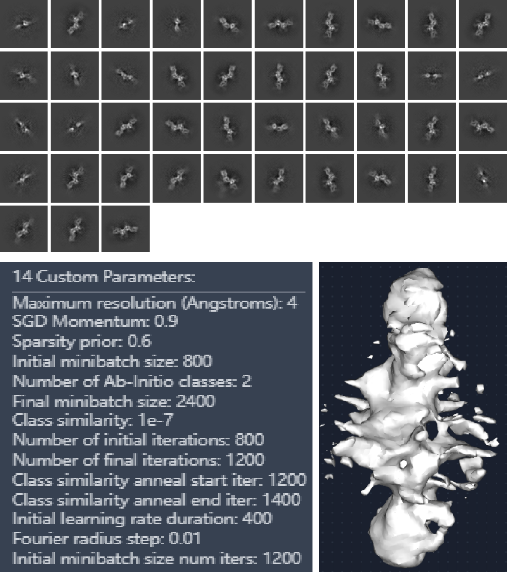
Those 2D classes do look promising! I wonder if you noticed though that along the edges of the class averages, there are thin spikes coming off your protein — kind of like a 2D version of the spikes you see in your ab initio model. The background region far away from the particles also has a texture to it, kind of like a waviness. Both of these are signs of overfitting.
Overfitting
Overfitting occurs when we don’t have enough true signal in our images, and so the algorithm starts to align noise instead of the particles. This is basically unavoidable — there will always be images or parts of images without signal in them, but the noise is everywhere. For a classic example of what can happen as a result of fitting to noise, check out the seminal paper from Richard Henderson. This is also why @Das recommended you don’t use your alphafold model to align your particles.
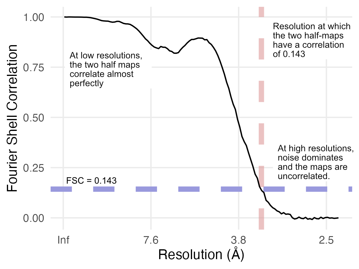
So now the question is, how can we be sure that what we see in our cryoEM maps is real, and not Einstein-from-noise? The field has settled on using something called Gold Standard Fourier Shell Correlation. This is quite a mouthful, and so you will often see it abbreviated as GSFSC or simply FSC.
For GSFSC we split the particles into two half sets. These half sets are used to create two copies of the map, but importantly the particles are never mixed up. This means we have two completely independent estimates of the 3D shape of your target.
The clever step is that we can compare these two structures at every resolution (see note at bottom). Provided that our particle stack is clean, we know that each half set should look exactly identical — there’s no reason that half-set A will have a different particle than half-set B. However, since noise is random, we expect the noise to be completely different in the two half-sets. Put another way: true signal should be highly correlated, while noise should be completely uncorrelated.
What we do is we look at the correlation for all of the different resolutions in our map. We then filter out (i.e., remove) the resolutions where correlation dips below some threshold. The choice of this threshold is somewhat arbitrary — the field has settled largely on looking at where the correlation drops below 0.143 and calling that the resolution. If you are interested in why 0.143 was selected, the Appendix of this paper lays out the (somewhat involved) argument.
How is this useful?
I’m telling you all of this because it’s important to know which jobs obey these rules and which jobs don’t. For example, 2D classification and ab initio do not use half-sets! This means they are susceptible to over-fitting and model bias. For this reason, they are generally treated as tools to quickly assess data quality or clean up junk particles, but once you have something that looks okay we recommend that users move on to jobs that do obey the half-set rule.
For instance, in your case, I would recommend you try a Homogeneous Refinement. This is a job that creates a single map of your particles, like ab initio, but it obeys the half-set rules. You might see those spikes disappear, or at least get a lot smaller and less intrusive. Homogeneous Refinement has some other tricks to reduce overfitting and can give quite nice results.
One more recommendation
Overfitting can also often be reduced by cleaning up your particle stack. The Heterogeneous Refinement job is really useful for this task. I bet you’d be pleased with the results of plugging in your particles from the ab initio job and two or three copies of your ab initio map. Hopefully you’ll end up with one cleaner stack of particles and two “junk” stacks which you can discard.
I put this recommendation in a separate section because Heterogeneous Refinement is another job that does not obey the gold standard half-set rules 
I hope this all helps! I know that’s a ton of information, but I hope you will find it useful as you keep processing data, and we’re always here and happy to help with questions you have further down the line!
Note: More precisely, we’re comparing spatial frequencies. In 3D Fourier space, a given spatial frequency is represented by a shell. Since we’re calculating the correlation of all of these spatial frequencies, we are calculating the Fourier Shell Correlation — the FSC!