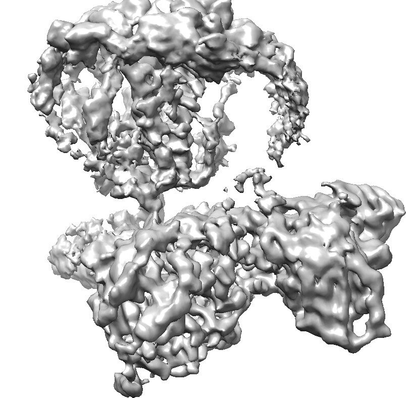
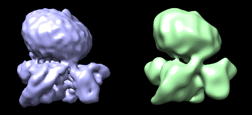
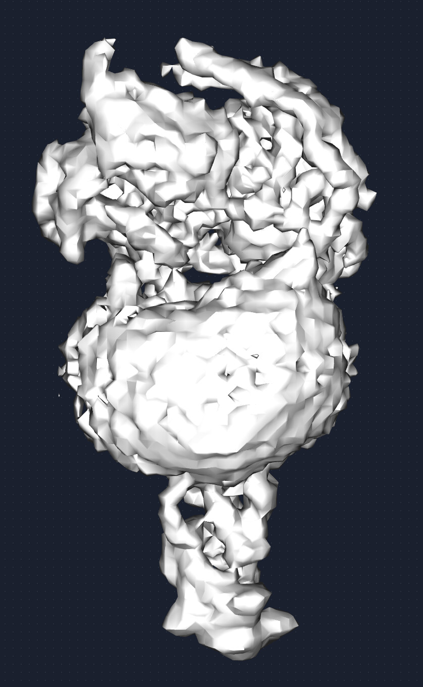
I recently processed a GPCR dataset. I used the topaz train and extract tool to pick particles, and remove the junk particles through 2D classification and heterogenous refinement. Then, I did the non-uniform refinement and local refinement. The reported resolution is around 1.68-2 angstrom, however, the map quality, as shown in the following picture, didn’t meet the expected standard for this resolution.
Particularly, the density of the receptor partition appears incomplete, with the micelle density still prominent. Now, I don’t know why the map is like this, and how to improve the map quality of the receptor.
I would greatly appreciate any suggestions you can provide. Thank you in advance.
How many particles? What does the FSC look like? What does the mask look like? What did the initial model you used look like? What was your processing strategy?
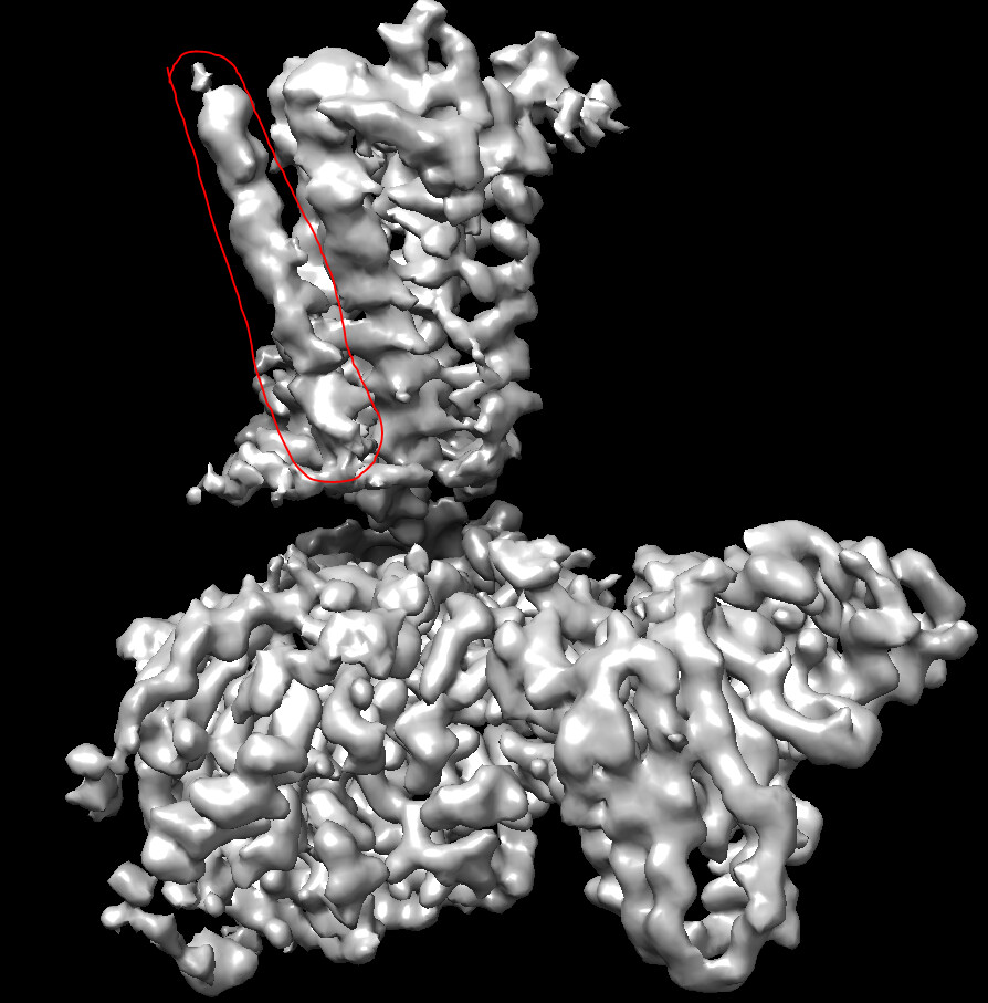
Hi, I performed heterogenous refinement further followed by the non-uniform refinement. The map looks better now, with a reported resolution of 1.68 angstrom. However, the density of a helix (circled in the red line) on the left side is not good, I don’t know how to improve this.
In addition, I have no idea whether this map quality already meets the reported resolution or not, although the local resolution estimation provides a similar resolution. Regradless, I still need a much higher-quality map to build an accurate atomic model. Therefore, what should I do to obtain a better map? Thank you very much.
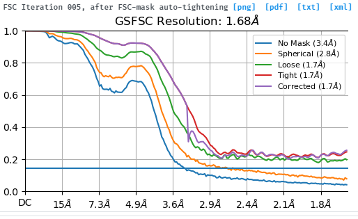
You almost certainly have a lot of duplicate particles in your data as the FSC curves do not fall to zero.
Remove duplicate particles, re-refine and you will probably end up with a structure at approximately 3.2-3.5 Å.
Once you’ve solved the pathological FSC curve, you can try CTF refinement (both local and global) to optimise electro-optical parameters, referenced based motion correction to try to push resolution further and local refinement (or 3D variability analysis/3D flex) to try to clarify weaker areas.
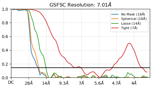
Hi, thank you for your quick response. I have two questions. I performed particle picking using the topaz tool and never picked particles on the same micrograph, if so, is it still possible to pick duplicated particles? In addition, why does the existence of duplicate particles boost the correlation between half maps, resulting in FSC curves not falling to zero.
What’s more, why do the ‘No mask’ and ‘spherical’ curves fall to zero but not ‘Loose’ and ‘Corrected’ curves? What’s the mechanism behind it?
I am really new to the single-particle data processing, so I am really need your generous help to understand it.
You’re working with a small membrane protein. If your micrographs are high concentration (particles close together) during classification they can be moved such that when re-extracted, two “different” particles are in the same place. CryoSPARC has some protections against this built in, but they’re not perfect, particularly if not remaining 100% in the CryoSPARC pipeline.
It’s made a little more complex by the fact that, by default, CryoSPARC does not “hard” classify (that is, assign one particle to only one class) during 2D classification or 3D heterogeneous refinement. If you select multiple classes from a heterogeneous refinement, there is a significant likelihood that particles will be shared between them unless you turn “hard classification” on.
Because you are comparing correlation between two halves of the dataset. If the same particle appears in both halves (because it is repeated) it will perfectly correlate to itself, artificially boosting the correlation between the two half-sets of the data.
The no mask and spherical curves do not fall to zero. They do fall below the FSC=0.143 line (which I do wish would be made a dotted line, but that’s a different issue) but do not reach zero.
The reason why the correlation is higher with increasingly tight masks is that the disordered regions (bulk solvent) are removed from the calculation. Bulk solvent is effectively noise… it’s a bit more complicated than that, but it’s not a level of complexity that really needs to be worried about for our purposes.
There are a lot of resources available for understanding cryo-EM image processing, from primary literature to YouTube videos, software documentation, forums and mailing lists. If using CryoSPARC, I’d suggest starting with their documentation. The relevant page on FSC is here.
Just recursively follow citations through and you’ll soon be down a very deep and very interesting rabbit hole.
I’ve noticed a couple things, working with GPCRs quite frequently.
GPCRs don’t work super well in 2D classification, especially the class A GPCRs that don’t protrude from the micelle on the receptor side. If you’re at high concentration, as @rbs_sci mentioned, it’s very easy for the 2D classification to move the particles around and end up with duplicates.
My preferred workflow for GPCRs is to collect the data, pick particles, select just the best couple classes, use those for a 2-3 class ab initio, then go back to the original picks, and do a het refine of all the original picks (pre-2D classification). Then take the best class from het refine, and either re-do het refine with just the particles that fall into that best class, or go to NU-Refine
You can get very spurious resolutions from NU-Refine with the Class A GPCRs because the micelle density seems to dominate the alignments if you don’t have great alignments to start with, and since those correlate just about anywhere and are a huge chunk of the density, I’ll commonly see a normal FSC curve that then pops back up and shows lots of correlation at high resolution. Such as:
The best solution I’ve found is to set the input volume low pass to something like 10 Å instead of the typical 30.
Thank you so much@rbs_sci. I really appreciate your explicit explanation.
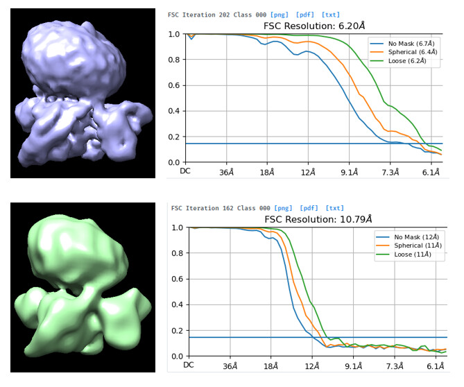
Now I am confused about how to remove junk particles correctly and effectively. I found that if I used the particles of bad classes from “output” of the first decoy hetergenous refinement as the “input” to run the decoy heterogenous refinement once more, some bad particles still can generate good volume (right side), though maybe not as good as the first time (left side).
Therefore, what are the good particles? What are the bad particles (junks)?
In addition, I found the other wired thing is that I ran the “topaz extract” job to pick particles on the micrographs where I ran the following bin4 re-extract from micrograph job, however, the latter one didn’t pick particles on more than 100 micrographs, missing many particles. Do you know what happened during the re-extract?
Thank you very much for sharing the valuable tips with me.
May I know which job you set the input volume low pass to 10 angstroms? And why does this will help the resolution? How does it help? Looking forward to your great ideas.
What was the resolution of the two classes? The definition of “junk” is still quite subjective and a little user dependent. For example, I’m more lenient than many regarding discarding micrographs because of several samples I’ve worked on in the past where even micrographs which estimate 8-10A CTF fit can still give decent results when all electro-optical refinements have been carried out on individual particles, but I’m a bit less lenient on bad particles and tend to clean my datasets extensively (multiple rounds of 2D-2D-3D-2D-3D-2D-3D as required).
Regarding Topaz, I’ve no idea what happened there - I rarely use it and thus far only in RELION.
Regarding the 10A lowpass, small proteins, particularly small membrane proteins, tend to align poorly at low resolution. This is because the detergent micelle dominates at lower frequencies and can mean particles end up misaligned, which results in a poor quality reconstruction.
They are bin4 particles, so the pixel size is 3.31 angstroms.
I am very interested in the experiences you mentioned above, where the 8-10 Å CTF fit particles still gave you great results when you optimized the electro-optical refinements. For me, I usually discard micrographs with a CTF fit worse than 6 Å . Therefore, may I ask what electro-optical refinement is? What jobs can perform these refinements? How do you test the electro-optical parameters during the refinement? It would be really helpful if you could explain them to me.
Thank you for sharing so much with me again.
It’s all the contrast transfer function variables (the influence of the electron optics of the microscope). Defocus, astigmatism, second, third and fourth order beam tilt, magnification anisotropy, Ewald sphere correction… (also Cs, and Cc, although that should be constant unless you’re swapping column hardware around or have a Cs or Cs/Cc corrected microscope!)
I work a lot with samples where I don’t get so many particles per micrograph (usually <10) so every micrograph I throw away really hurts. For small samples, I can be a lot more particular, and 6A is not a bad cutoff to use… some would recommend higher still. It will depend on what you’re working on!
The second map looks like it contains duplicates because the FSC does not reach zero despite the low resolution estimate, but the first map hits (or is very close to) binned Nyquist so I’d unbin that (maybe to bin2) and do a NU refine run, see what it gives.
If the particle count is not so high, I would then create templates and repick all micrographs and redo 2D classification, then heterogeneous refine with two copies of the good map and one “junk” class (not that 10A map, it has too many features).
I had a quick experiment with 400 micrographs from EMPIAR-10673 last night out of curiosity, and leaving the default lowpass of NU refine at 30A or decreasing it to 15A made no difference in the final result, but the 15A initial lowpass converged more quickly (bin3 so Nyquist was ~6A):
Thank you for the explicit explaination and suggestions.
So would you like to run the CTF (local or global) refinements to find the correct parameters for indiviual particles, or do you have your own skills?
To the point you mentioned, the detergent micelle dominates at the low frequencies, leading to particles being misaligned. My question is: which part of a sample (including the protein of interest and solution) is supposed to dominate at low frequecies, and conversely, why are the other parts supposed to dominate at high frequencies? When cryosparc programs calculate the particles alignments or reconstruction, which signal does it use–Fourier transform space or real-space? To be honest, I don’t understand the relationship between the Fourier space and real-space for a particular particle, such as which part of the particle corresponding to the high or low frequecies of its Fouries space? and why? Is it because of the conformation stability or homogeneity?
The class B (such as EMPIAR-10673) are much easier to align, because of the extracellular receptor extension. The class A (like what I think Jianming has) typically align worse in my experience, although it depends on a number of factors such as the specificity of the ligand.
For smaller proteins, if they are in a micelle, the relative percentage of the signal from the micelle is higher than if it was a large complex. As the micelle is disordered, this can cause problems.