Case Study: End-to-end processing of an inactive GPCR (EMPIAR-10668)

[hbridges1]

Hi CryoSPARC users! We are excited to share with you a new end-to-end data processing case study of an inactive GPCR (EMPIAR-10668) that you can follow along with!

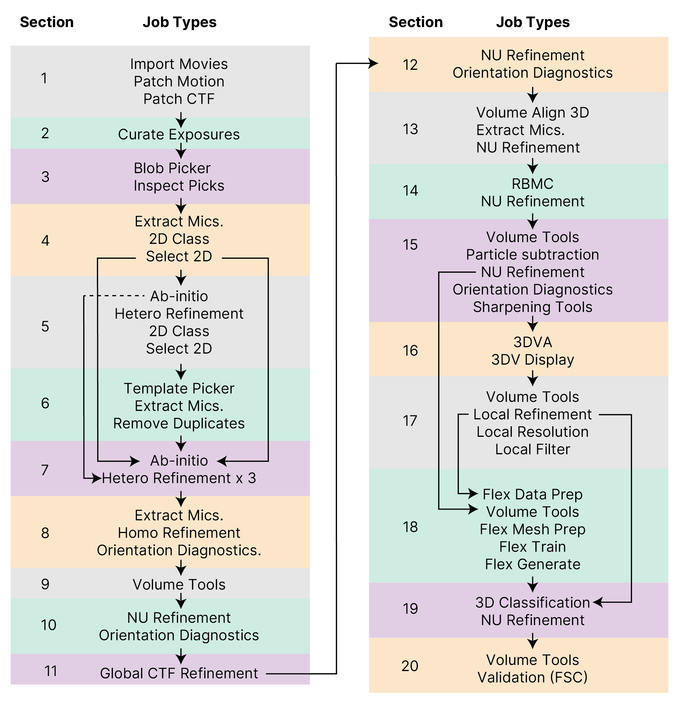
Here we guide you all the way from downloading an EMPIAR dataset through to generating maps ready for model-building, as well as analysing and separating states within a continuous motion. Our final sharpened maps, half maps and masks are downloadable to allow comparison with your results.

This case study is of a relatively small membrane protein target at 73 kDa, and within the complete processing pipeline it includes ideas on how you might handle:

• crowded or loosely associated neighbouring particles
• assessment of auto-masking and auto-sharpening
• resolving flexibility of a small subdomain
• cross-verification of 3D Flex results

We hope this detailed guide is a useful resource for users old and new! Let us know of any other types of targets, or particular single particle cryo-EM challenge that you would like to see a case study on in the future!

[olibclarke]

This is great Hannah!! Particularly like the clear and detailed description of how to apply 3D-flex, and the emphasis at the end on double-checking masks (Case Study: End-to-end processing of an inactive GPCR (EMPIAR-10668) | CryoSPARC Guide)

In this instance, did 3D-flex reconstruct help improve the density locally or globally beyond what could be accomplished by local refinement? Or it was mostly useful for analyzing/describing conformational heterogeneity?

[hbridges1]

Thanks @olibclarke! I’m glad you like it.

That is a great question about the Flex analyses! In this case, 3D Flex was used in order to analyse conformational heterogeneity. We found Flex Reconstruct improved the density of the extracellular domain relative to the input volume (not included in the case study), but the best quality density for this domain was found in the classified and re-refined ECD rotation class 1.

[olibclarke]

Thanks! I’m also curious about the subtraction step:

In the case study, you use an inverse mask to subtract low threshold density outside the main volume. Where is this density coming from? Adjacent particles, other junk?

I wonder if you considered using a complimentary strategy: What happens if you subtract the density of the GPCR, and then 2D classify the resulting particles - perhaps this will allow you to identify the particles that are causing this (presuming that it is just a subset of particles). You can then revert to the unsubtracted particles after removing the offending junk-containing subset - we have seen cases where this works quite well. The nice thing is that the subtraction in this approach tends to work pretty well, as by definition your high res GPCR is pretty well-ordered and matches pretty well to the projections you are subtracting.

Cheers
Oli

[hbridges1]

Thanks for these questions @olibclarke!

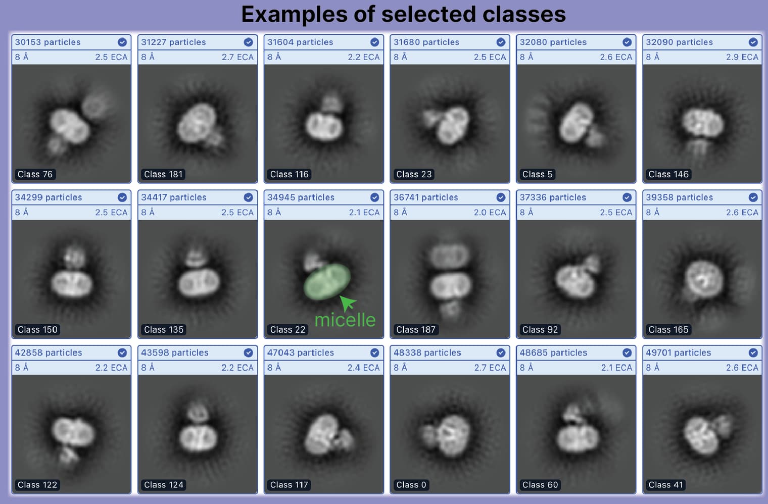
During 2D classification with the default circular mask diameter, we see classes where adjacent particles are clearly visible (for example in Figure 3 highlighted in yellow), so there may be a somewhat ordered association between nearby extracellular domains, and it seems likely that the additional density comes from adjacent particles.

Thank you for outlining a complementary strategy that might help with the superfluous density. We have not tested such a procedure on this dataset, but it is a really interesting idea for us or others to try!

[olibclarke]

Ah I missed that, thanks Hannah!

I see what you mean - yes looks like interacting particles interacting in multiple different ways - in these kinds of cases (overlapping/interacting/aggregating particles) we have sometimes found it helpful to subtract the main particle, then classify on the residual background to identify a clean subset (but like everything in cryoEM it seems, just one of those things to test on a case-by case basis )

Thanks again for this very helpful & comprehensive workflow!

Cheers
Oli