Hi everyone,
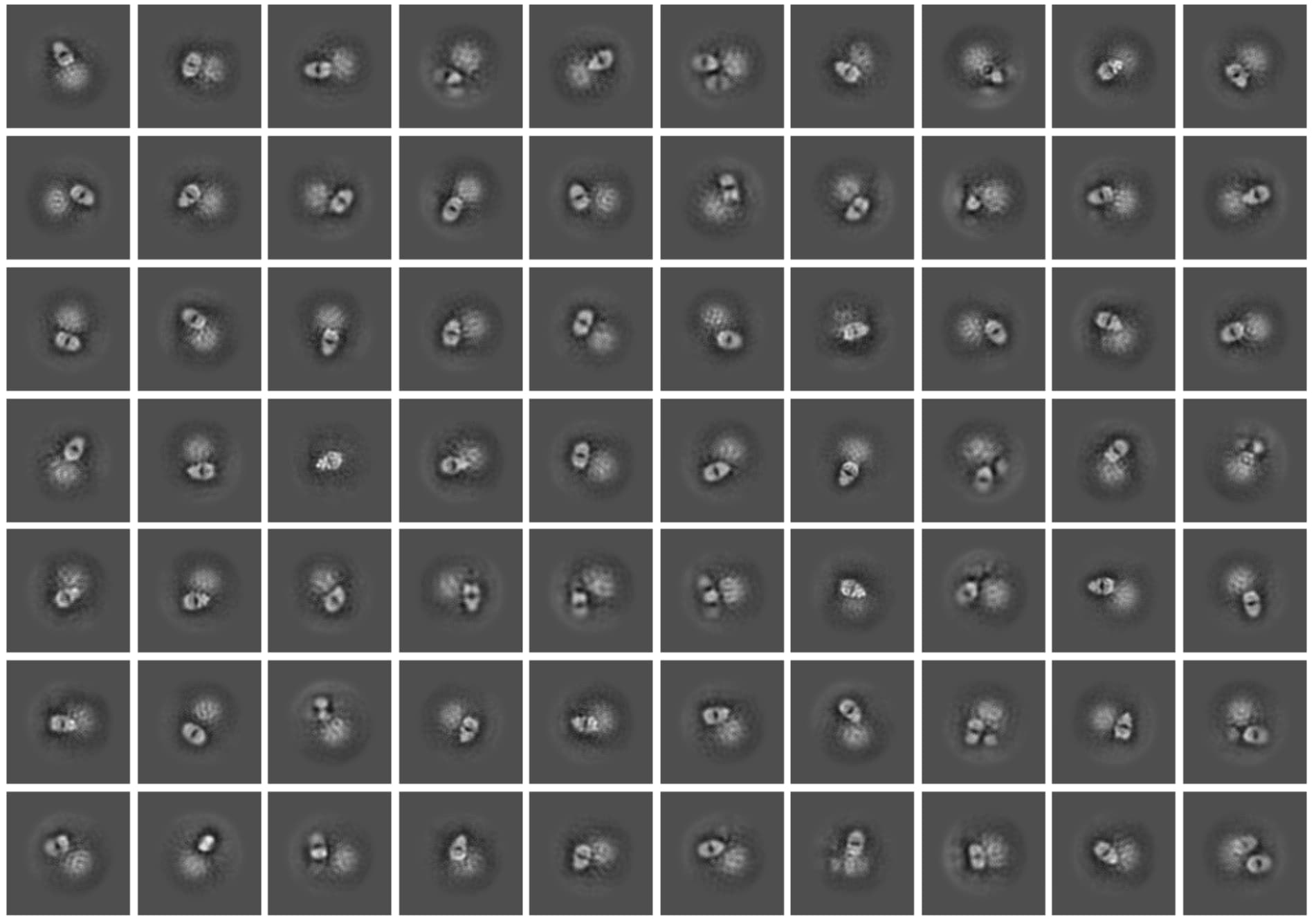
I am working on a small membrane protein (25Kda). We have a antibody that specifically bind to a cytosolic loop of the membrane protein. We recently prepared a protein-Fab complex (25+50=75 Kda in total) and collected some data with Krios. I can clearly see the feature of Fab in 2D classification, but the density of membrane micelle looks really smear, doesn’t look like a typical detergent micelle actually:
I also tried some ab initial, the Fab region looks good but I can’t see anything inside the detergent micelle. Also, it seems that the orientation between membrane protein-Fab is very flexible as I can see multiple conformation in ab initial. Is this because of that the particles are not well aligned? Which is due to the inherent flexibility of the complex? Anything I can do to improve it? Any suggestions and questions are welcomed, thank you in advance!
Best,
Yan
Hi Yan,
I haven’t worked with membrane proteins, so hopefully someone else comes along that can recognise what’s going on.
However, I’m curious to hear if you purified the Ag-Fab complex before applying it to the grid, such that there should be minimal free Fab on the micrographs. Assuming the splotches next to the well-aligned Fabs are micelles with your Ag, it seems like the same projections of the Fab have the Ag sitting on different sides of your Fab, meaning that the paratope would have to be all over the place.
Fabs always give very strong features in my experience, so actually I would expect to see something like this from a grid with a lot of free Fab and high particle density such that every Fab has neighbours that become diffuse averages in 2D classification. Could you maybe show a motion-aligned, representative micrograph?
Hi Martin,
Thank you so much for your reply. I do purify the Ag-Fab complex by using gel filtration before applying it to the grid. My protein is easily to aggregate, so I used fresh purified, un-concentrated sample and continuous carbon grid.
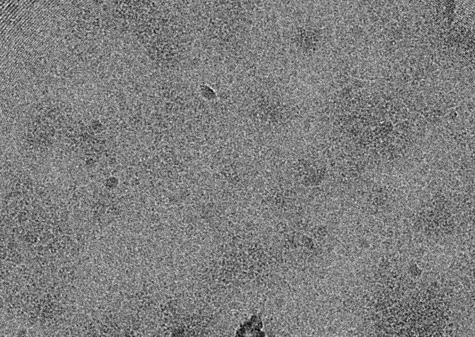
Yes, you are right: The particle concentration is very high in the raw image:
And although I am using purified complex, I do see some classes that looks like Fab alone at the beginning of 2D classification. This is a little bit confusing to me.
For now I am using a relatively big box size to extract the particle (400px, pixel size is 0.84). Should I try to use smaller box size for such crowded sample?
Best,
Yan
Hi Yan,
It’s completely normal that some of the Fab will dissociate during blotting, so seeing some free Fab classes is to be expected. Still great that you are separating out the free Fab before application to the grid, since otherwise the actual Ag-Fab picks would most likely drown in free Fab picks and be distributed like junk.
This might not be the most popular opinion on a processing forum, but personally I would probably try to get new data from grids with a lower protein concentration. Even if you don’t have a lot of particle overlap, and the signal might be there as is obvious from your beatiful Fab 2D class, the processing has gone much more smoothly when I collected new data from grids where I could actually tell by eye where I had particles. Could you try and show a micrograph taken further from focus? Or just a cherry-picked micrograph with a lower particle density?
Are you sure you’re using continous carbon? Since you’re working with quite a small particle, you’ll get very low contrast on continous carbon, so it might be a bit optimistic to use that substrate. Have you tried applying graphene oxide to a holey carbon grid instead?
If collecting new data was out of the question, I would maybe try to group the 2D classes into superclasses using the “Rebalance 2D Classes” job without any rebalancing and then do further 2D classification within the superclasses to see if I could find any ordered signal within the diffuse splotches (preferably for the ones where the diffuse signal is close to the Fab paratope). Like I said, though, I would personally go for new data, so I don’t have a lot of experience working with such crowded micrographs.
It’s possibly that using a smaller box size or just a tighter mask could help a bit, but it already seems like the 2D classes are picking up on the Fab and something else, without much signal from anything further away. Anyway, there are a lot of cases where things are mysteriously improved by changing to box size in either direction and it’s fast to try, so why not…
I agree with @au583982 about collecting new data, unfortunately. I’ve worked with membrane proteins, and this micrograph reminds me very much of when my grids were far too crowded.
Could you let us know what concentration (in nM) you applied to the grids? In my experience, continuous carbon requires orders of magnitude (~100 times) less protein than normal holey carbon (e.g. quantifoil) when working with membrane proteins.
If you do want to go ahead processing this data, it is somewhat concerning to me that the Fab adopts so many different conformations relative to the blob present in the rest of your data. Have you tried ab initio with multiple classes? Could you show us what your ab initio results look like?
Hi Martin,
We used focus from -1.5 to -2.5 during data collection. The image I showed you is -2.52, which is already the furthest one from focus. And the particle density is basically same in all the images. I think we have Graphene Oxide on Quantifoil® R1.2/1.3 here, but we haven’t try it yet.
We can definitely try to collect new data, and probably that’s the best way! Maybe we can try to concentrate the protein a little bit and try regular quantifoil grid. But in the meanwhile, I will try what you suggested and see if anything changed.
Thanks again for your help!
Best,
Yan
The concentration is about 0.3 mg/mL, which is around 4000 nM. I will definitely try to prepare new grid, using lower concentration for continuous carbon or try regular quantifoil grid.
As you said, it is concerning and I haven’t done too much with ab initial yet, here is 2 classes from about 40k particles:
And I have a naive question: how does crowded images lead to this? I thought it would be difficult to pick particles in very crowded images, but I do see some very clear Fab by itself. Thanks!
You’re definitely right that I unfortunately don’t have a great theoretical explanation of how you can pick Fabs if it truly is too crowded. I just remember my ice looking like this before I had dialed in a much lower concentration for my good grids.
Specifically, I am referring to the fact that there are no clear regions of your micrograph which are “empty” or “flat” — basically every region has at least some kind of “texture” to it, and some parts have even more texture. I know this is not very formal, but it’s just my intuition.
One thing I’m noticing is that you still have quite a few particles in each 2D class. I generally try to shoot for ~200 particles per class, or however many my GPUs can handle (typically the latter is the limitation these days). I might try performing classification with as many classes as you can to see if something interesting falls out.
I’d try to keep classes with the “blob” in the same position relative to the Fab, if you can, just to see if there really is structure there. One thing that could be happening is that your grid is so crowded that it’s aligning to whatever nearby high-contrast feature is available and not whatever the Fab has bound.
To speed this process up you can reduce the alignment resolution. You might also consider increasing the Initial Classification Uncertainty Factor, since the Fab will always look the same and we care about the less-ordered stuff nearby.
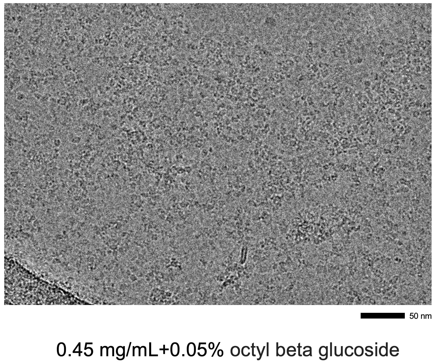
A quick update:We reconstituted this membrane protein into nanodiscs and tried cryo-EM. This complex is easily to aggregate or break during freezing. We overcame it by adding 0.05% octyl beta glucoside into sample right before freezing and it helped.
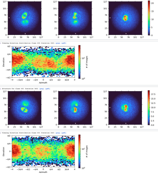
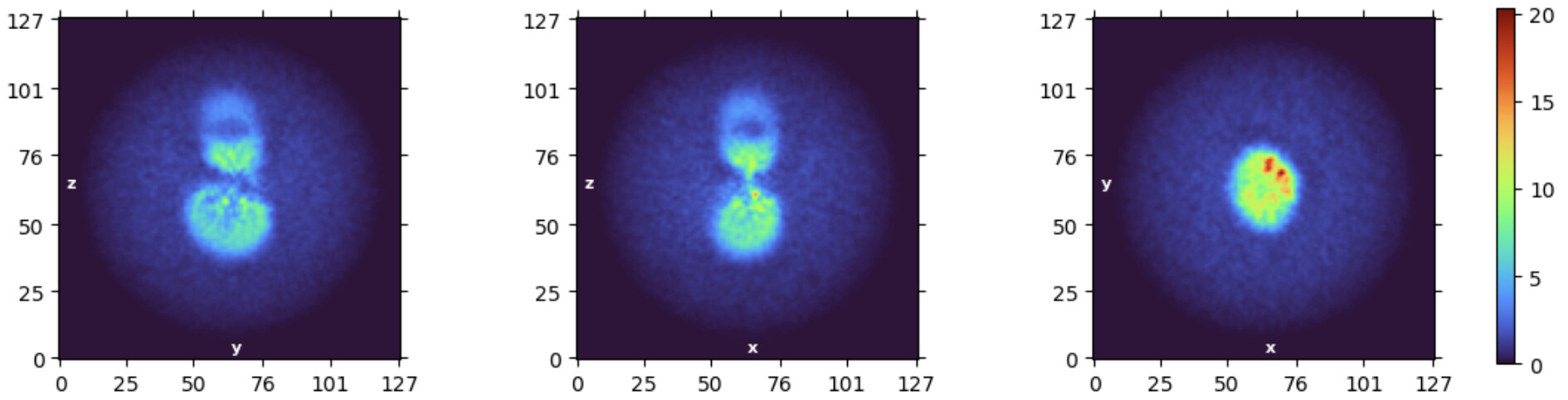
We performed ab initio with ~25k particles, unfortunately we didn’t see any protein signal from the disc. We plan to run hetro-refinement with all the particles (~65k) but don’t know how it will end.
Hi @wangyan16! These definitely look better than the ones you posted a few months ago! I think it is especially promising that the classes where the Fab is “sideways” compared to the nanodisc are mostly gone.
If you do get anything with promising low-res density inside the nanodisc, I definitely would recommend a local refinement. This will let you mask out the Fab so that the alignment focuses on just the part you are interested in!
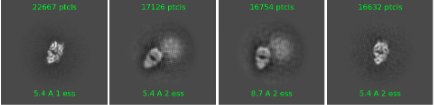
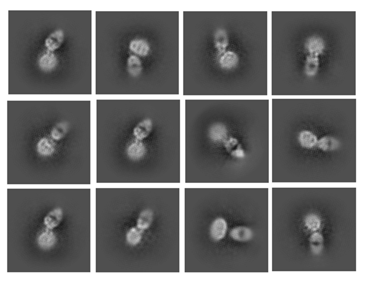
Yes, we do start to see some signal from the discs! After further cleaning up, we have about 100k particles left, here is the typical 2D classification:
However, due to the limited particle number and small size of the target protein, we are not able to see some real structure yet.
Thank you for the suggestions of local refinement! Can I simply create a mask in chimera by eraser? Beside the Fab, should I also exclude the density that are potentially MSP that outside the nanodisc?
Awesome, that is exciting news! This looks like a challenging target, so you’ve made great progress so far! Hopefully we can squeeze out a bit more from these 100k particles, but you may need more data.
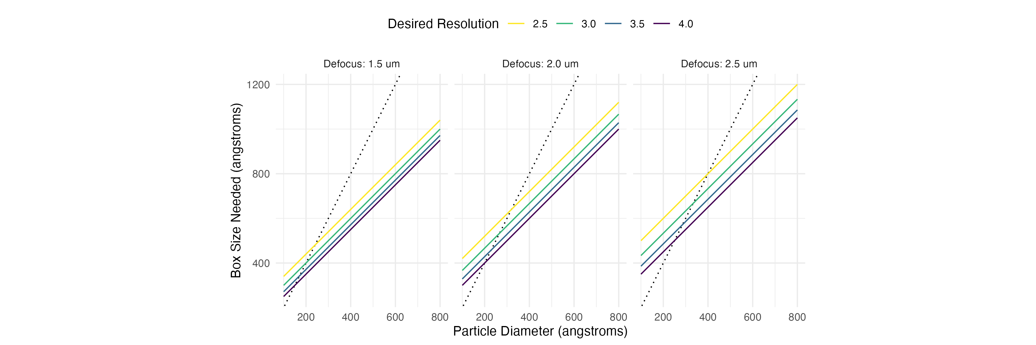
You might also want to consider extracting with a bigger box size. With such a small particle, the normal heuristic of 2x the largest diameter doesn’t quite work. A better box size is given by
This formula is given in the classic Rosenthal and Henderson 2003 in JMB. When your particle is large, using the 2x particle diameter estimate gives a sufficiently large box, but with smaller particles it is better to go a bit over that size, especially if you have high defocus and your data goes to a high resolution.
Here is a plot showing a few particle sizes, defocus values, and the recommended box size for that combination. I’ve included the 2x particle diameter line in each plot for reference as a dotted line.
Yes, you can use Volume Eraser to make a mask for this target. We have more advice on mask selection and creation in our guide. Be sure when you re-import the mask that you give a nice soft edge so that you don’t run into alignment issues due to ringing artifacts!
For your target, since there is so little to align, I would include the nanodisc for now. It will provide a nice large low-resolution signal to aid alignment. I would also recommend turning on a Gaussian prior for your local refinement. This will make the algorithm “prefer” alignments which don’t move the particles very much. This can help avoid overfitting when you are masking out a small target.
Please let me know if you have any more questions!
Hi @rwaldo , The box size is 320 and pixel size is 0.84, I guess it should be good for this small protein with diameter of ~8 nm.
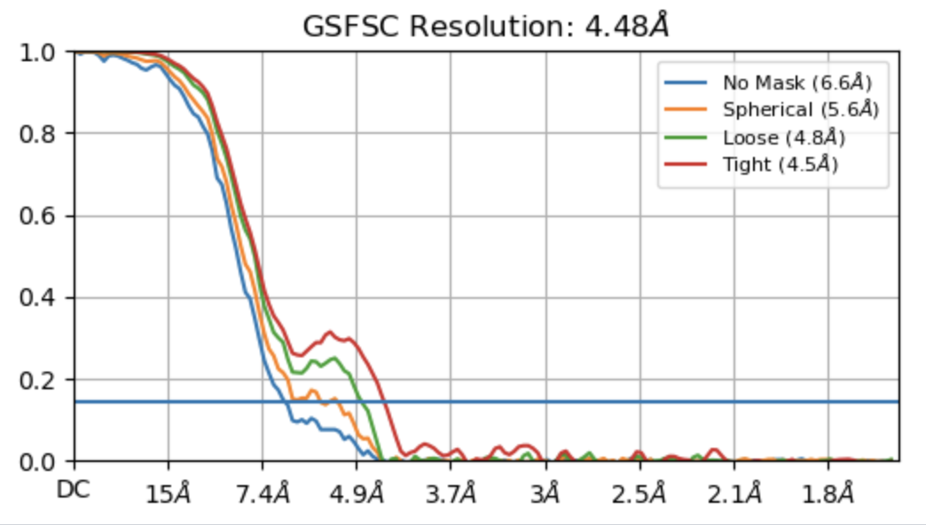
I created a mask that covers the disc region by using segger and performed local refinement. The GSFSC doesn’t look too bad, and did help to improve the resolution from 6.5 to 4.7.