Add CTF effect to projections of a volume

CirenSangzhu · September 16, 2022, 2:34pm

Hi guys! I’m quite new to cryoEM, and I’m playing with CTF and cryoSPARC Simulate Data (BETA) job, but I find that results of my own CTF code are quite different from the ones cryoSPARC Simulate Data (BETA) job gives. As I can only post one figure, I combine all figures in one and insert it at the end.

Here is the thing. I want to get some clean projections of a volume first (this can be done by cryoSPARC or other softwares like RELION, EMAN2, etc), and then add CTF effect with given parameters to these projections. To my understanding, this can be done by taking the Fourier transform of a projection, multiplying the 2D CTF image in Fourier space, and doing the inverse Fourier transform.

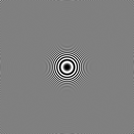
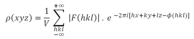
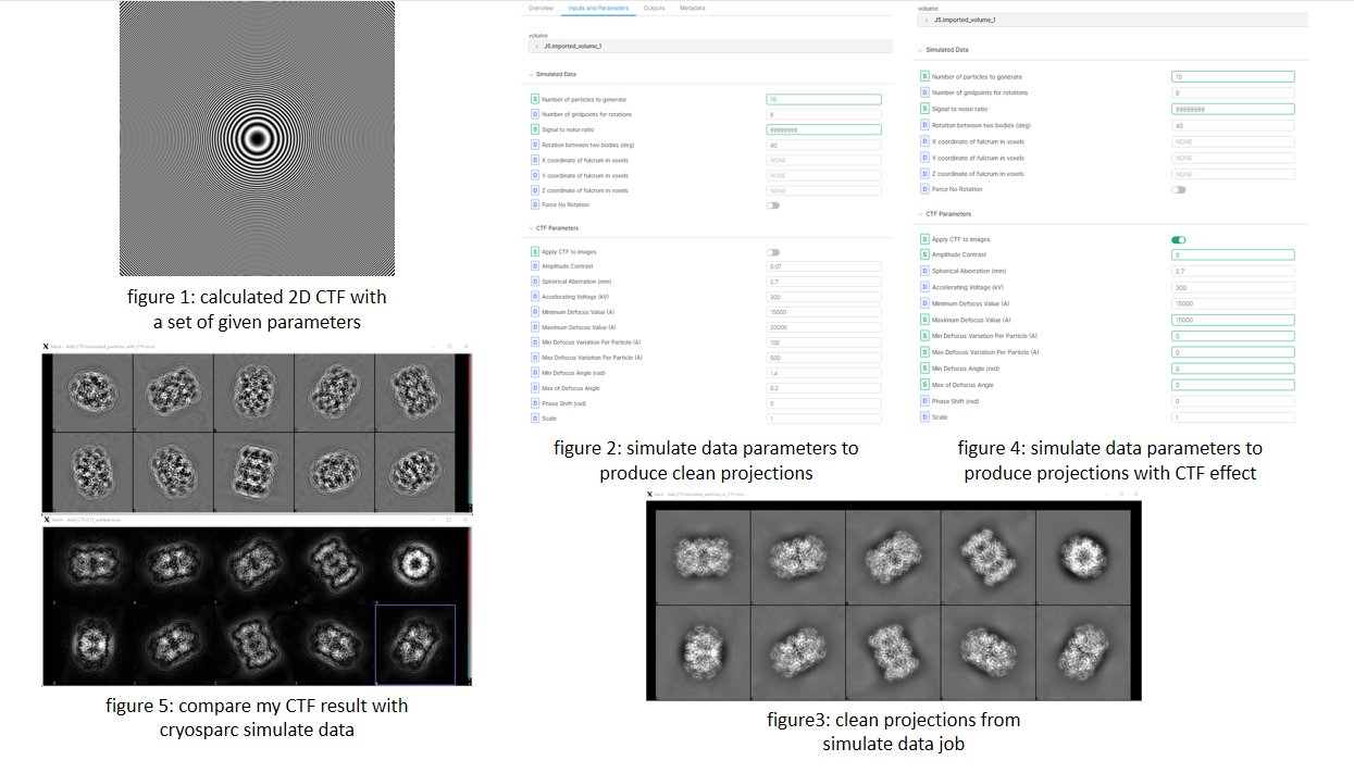
So, I calculate the 2D CTF image according to the CTF formulation. ( [CTF Estimation - CryoSPARC Guide]) It looks like figure 1 with parameters: defocus=15000 angstrom, voltage=300kV, Cs=2.7mm, phase shift=0rad, pixel size=0.6575, image size=440. The first 4 parameters are sufficient to calculate CTF value according to the formula on the website, and the last 2 parameters are consistent with the imported volume.

Clean Projections of the volume are produced by cryoSPARC Simulate Data (BETA) job. I set the SNR to a really really big value, and turn off the CTF option. The overall parameters are shown in figure 2. I think the result particles are very close to clean projections of the imported volume, as shown in figure 3. (It’s viewed with EMAN2 e2display.py)

To add CTF, the .mrcs file is read by mrcfile python package firstly, and CTF effect is added to the projections by numpy as:

mrc = mrcfile.open(file_name, mode=‘r’)
data = mrc.data
mrc.close()
proj = data[k, :, :] # shape (440, 440), k iterates over all projections
ctf_2D = … # ctf_2D is the one shown in figure 1
proj_with_CTF = np.abs(np.fft.ifft2(np.fft.fft2(proj)*np.fft.fftshift(ctf_2D)))
CTF_added_proj_stack[k, :, :] = proj_with_CTF
… # write .mrcs file with CTF_added_proj_stack

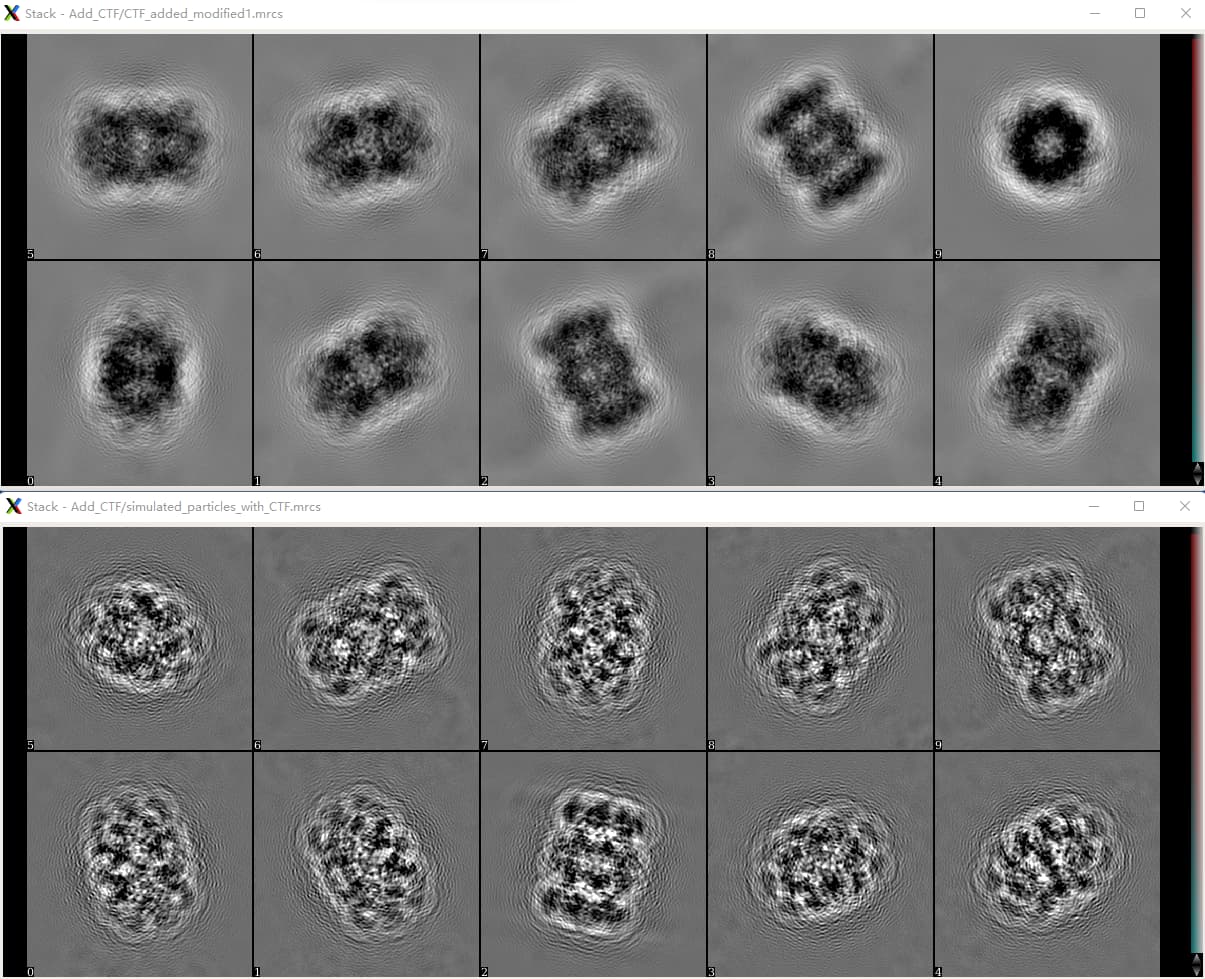
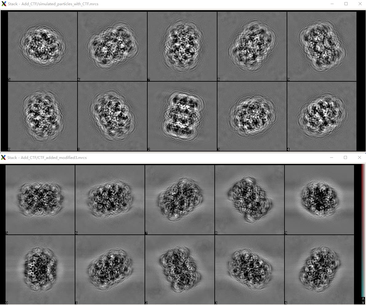
When I turn on the CTF option in Simulate Data (BETA) job, set the CTF parameters the same as used in my own code, and remain the noise parameters the same, I also get the projections affected by CTF. (Overall parameters are shown in figure 4, and I think it matches the parameters used in my code, which is described above to produce figure 1) As shown in figure 5, however, comparing the results of my code (figure 5 bottom) and cryoSPARC Simulate Data (BETA) (figure 5 top), there exists significant difference. (viewed in EMAN2 e2display.py)

I have tried but can’t figure out what’s wrong. I also tried to use projections produced by EMAN2 and add CTF effect by my code, but the results are similar as described above.

Why is it? Do I make mistakes on data processing or CTF calculation? Or do I miss some steps to add CTF effect? Anyone can help me? Thanks for any suggestions!

Cheers
Ciren

CirenSangzhu · September 16, 2022, 2:37pm

The CTF image (figure 1) is not correct after posted, probably because I take a screen shot to make this combined figure. It’s quite different with the original image. I try to upload the original CTF image here.
figure1-CTF

CirenSangzhu · September 16, 2022, 2:38pm

Yep, this one looks good!

mmclean · September 16, 2022, 2:52pm

Hi @CirenSangzhu,

In the simulate data job, the CTF is indeed applied by multiplying the Fourier-space projections of the volume by the CTF, then transforming back to real space. However, the particles are also then multiplied by the scalar blob/sign value found in the output dataset. By convention, this -1 in order for particles to visually appear as “dark-on-light” (at least at the lowest frequencies).

Your process looks correct except for the use of np.abs on the projections – this isn’t done in our simulation. Do you see that the discrepancy is eliminated if you remove the call to np.abs, and instead just multiply the projections by -1 before plotting?

Best,
Michael

DanielAsarnow · September 16, 2022, 5:16pm

@CirenSangzhu You may enjoy this simple notebook (and the called code in the main pyem repo).

github.com

asarnow/pyem-nb/blob/master/BasicProjection.ipynb

{
 "cells": [
  {
   "cell_type": "code",
   "execution_count": 12,
   "id": "5199c856",
   "metadata": {},
   "outputs": [],
   "source": [
    "import matplotlib.pyplot as plt\n",
    "import mrcfile\n",
    "import numpy as np\n",
    "import pyfftw\n",
    "import pyfftw.interfaces.numpy_fft as fft\n",
    "import seaborn as sns\n",
    "from pyem import ctf\n",
    "from pyem import geom\n",
    "from pyem import vop\n",
    "from pyem import star\n",
    "pyfftw.interfaces.cache.enable()\n",

This file has been truncated. show original

CirenSangzhu · September 17, 2022, 10:17am

Thanks for you reply! @mmclean

I get the idea of blob/sign and know how it affects the plots according to your explanation! Thanks! Also, I take your suggestion of removing np.abs. So, my code of applying CTF now looks like:

mrc = mrcfile.open(file_name, mode=‘r’)
data = mrc.data
mrc.close()
proj = data[k, :, :] # shape (440, 440), k iterates over all projections
ctf_2D = … # ctf_2D is the one shown in figure 1
proj_with_CTF = -np.fft.ifft2(np.fft.fft2(proj)*np.fft.fftshift(ctf_2D))
CTF_added_proj_stack[k, :, :] = proj_with_CTF
… # write .mrcs file with CTF_added_proj_stack

Indeed, the results of my code get better, at least the backgrund looks better. However, they are still quite different from the cryoSPARC simulate data job results. The following figure shows the difference. Top is the results of the modified code, while the bottom is the results of cryoSPARC simulate data job.

Does my modified code meet take your suggestion correctly? Or is there any other mistake?

What’s more, I have another question of removing np.abs. To my understanding, np.fft.ifft2 results in a 2D array containing complex number. Then, without np.abs, CTF applied projections are complex matrix. I’m confused, because I think elements in .mrcs file are real numbers. (Though there is no error
arised when I write the complex matrix proj_with_CTF to a .mrcs file using mrcfile python package)

Thanks and Looking forward to your reply!

Best,
Ciren

CirenSangzhu · September 17, 2022, 11:40am

Thanks for your reply! @DanielAsarnow

I check the provided notebook, and browse the pyem repo. By the way, it’s really a great repo containing many useful functions. Thanks!

Back to the problem. I haven’t clearly understood each called main pyem repo code in detail, but in the notebook, it makes a projection of a volume in Fourier space, then transforms it into the real space. After that, CTF is applied to the projection by multiplying 2D CTF and Fourier slice.

In my case, I start with a clean projection in real space rather than Fourier space, so I apply CTF to the projection using the code in the original post. I haven’t clearly understood the code of getting Fourier slice in pyem, but I noticed that the notebook uses np.fft.rfft2/np.fft.irfft2 rather than np.fft.fft2/np.fft.ifft2. Is this the key to my problem?

I change my code and try this to apply CTF:

proj_with_CTF = -np.fft.fftshift(np.fft.irfft2(np.fft.rfft2(proj)*np.fft.fftshift(ctf_2D)[:, -221:]), axes=1)

The outermost np.fft.fftshift with axes=1 is to make the results look fine, though I don’t know why. The - sign is according to @mmclean blob/sign. The [:, -221:] is to match the shape of np.fft.rfft2(proj). I don’t know whether the code is correct, but it does give a result, as shown in the following figure. Top is the result of cryoSPARC simulate data, while bottom is my result.

It’s difficult for me to judge the result, but I feel there is still something wrong. Do you have any suggestion? Is it possible to realise applying CTF to a projection in real space with just a few lines of code and only numpy package rather than lots of other package? Thanks!

Best,
Ciren

DanielAsarnow · September 19, 2022, 3:27am

I start with a clean projection in real space rather than Fourier space

Once you understand the projection-slice theorem, I encourage you to use Fourier slices instead. Many things are simpler to understand and implement starting from Fourier space.

I noticed that the notebook uses np.fft.rfft2/np.fft.irfft2

Real signals have Friedel symmetry: f(i,j,k) = f(-i,-j,-k). Thus we can use the specialized FFT functions for real arrays, which save memory and time by computing only one unique half of the FT. Experiment: look at the array shapes and 2D sections of the rfft outputs, it will begin to make sense.

The outermost np.fft.fftshift with axes=1 is to make the results look fine, though I don’t know why.

The FFT algorithm computes the coefficients in a certain order. First, is the 0th coef, then 1, 2, 3, …, until N. Then it does the negative frequencies -N, -(N-1), -(N-2), … , -1. fftshift (and its partner ifftshift which is the same for even-sized arrays) swap the half-spaces along each axis, so that the order is instead -N, …, -1, 0, 1, …, N. Experiment: Transform any real-space image, and then back-transform again. Only one order of using fftshift will let you arrive at an image that is numerically identical to the original. (Hint: you will need to shift twice).

My Fourier-slice code works with the real transforms, in the conventional frequency order, but the CTF code is agnostic. It computes the CTF on the frequency grid that is given, regardless of its shape or order. By using the fftfreq and rfftfreq methods, we can get grids that already match our transforms. This is the most convenient and efficient way - you can see that in my code, only one Fourier shift is required at the end.

I don’t know whether the code is correct, but it does give a result, as shown in the following figure.

If the code is correct, your output will look just that from cryoSPARC, or pyem, or Relion. I can’t quite tell if you still have a contrast inversion or not because there are also some artifacts that look like some kind of interpolation error or from computing the CTF incorrectly.